Before beginning let me tell you that this is not a mathematically rigorous proof or explanation of CLT (central limit theorem). So chill guys! And enjoy the ride. I understand things better if I can get an intuition of the stuff, especially accompanied by pictures or figures. It may not be the case always with mathematical concepts. But CLT is one which you can visually understand.

Let me first request you to see this animated video which explains the essence of CLT :

(Please note that this video was not created by me. Credits go to the respective creators. I am just referring it here because it is so cute and relevant.)

There were articles about CLT in steemit before by @krishtopa and @joseferrer. You can see those articles in the below links:
https://steemit.com/popularscience/@krishtopa/fundamentals-of-the-central-limit-theorem-and-the-mysterious-law-of-large-numbers
https://steemit.com/mathematics/@joseferrer/mathematical-explanation-normal-distribution

Let us get started! What is Central limit theorem after all?

I will explain first using some statistical jargon. Don't worry. I will also explain it visually later.

Suppose if you have 'N' random variables (assuming N to be sufficiently "large") $X_1,X_2,X_3,...........X_N$ where each individual has their own probability distributions. And now if you add these random variables, the resulting random variable will exhibit the famous bell-shaped Gaussian distribution. (Instead of adding, finding the average of these random variables will also work. After all, averaging is also addition only. But after you add the variables, you divide by the total number of variables. :P The Gaussian distribution of your result for averages will be Normal distribution. The normal distribution is the normalized Gaussian distribution. That is the mean would be 0 and variance would be 1. Normal distribution is written as N(0,1))

Whatever I wrote above can be compressed in math as below:

$c=$PDF(\sum\limits_{i=1}^N X_i / N) = N(0,1)$

Those who don't like math can neglect it. Also, I have neglected some mathematical details regarding the choice of random variables above. That is not important for now anyway. But those who need rigor may ask in replies. :) I am happy to respond to those.

Now Comes the Visual part!

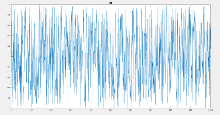
Think some random sequence of numbers. And for convenience let us say the numbers vary from -1 to 1. Also, let us say that the probability of occurrence of numbers which appear between -1 to 1 is the same. Let us call this random variable X1. So X1 can have numbers between -1 to 1 in its series and each number is equiprobable to occur. Now we have defined a random variable X1 which has a uniform distribution. There are 1000 numbers I am going to generate which are between -1 to 1. See below:

Let us see how the PDF(X1) (Probability distribution function of X1) looks like:

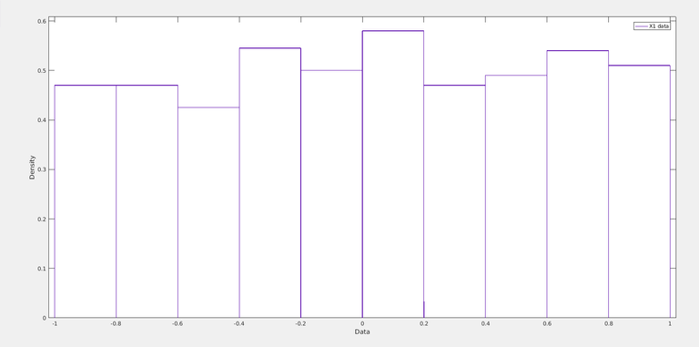
Yeah, it is more or less flat. Ideally, if the numbers are infinite it would be a dead flat distribution. This is approximately uniform distributed.

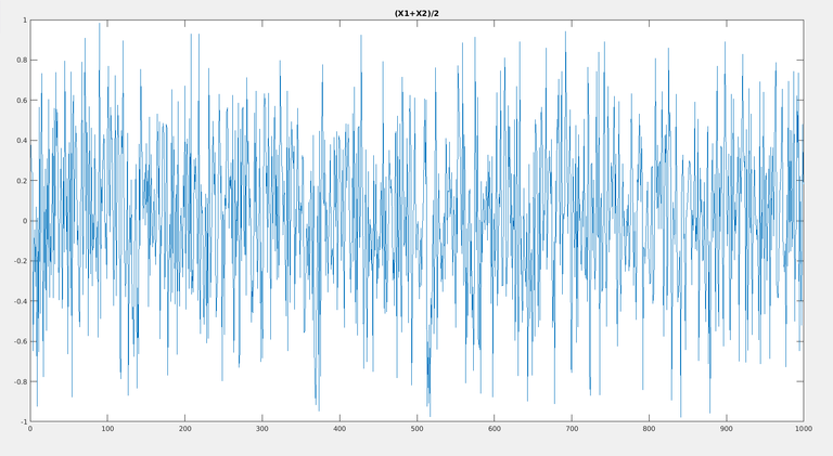
Now let me create X2 another random sequence with same properties of X1. The distribution must be similar, but the X1 and X2 are different sequences, although the statistical properties are same. So let us plot (X1 + X2)/2 next. (X1 + X2)/2 is the average of X1 and X2.

Pause!

Now just pause and think for a moment. Can you predict what can be the properties of (X1+X2)/2
So you can naively say that there would be more values near the zero. Because numbers are more to get canceled here.

Let us see anyway. Adding X1 + X2 gives the plot as below:

And PDF((X1+X2) / 2) looks like below :

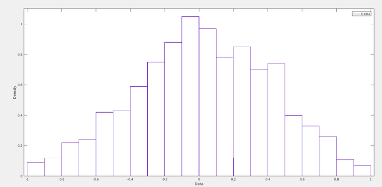
The distribution is triangular, suggesting the probability of values getting near zeros at greater.

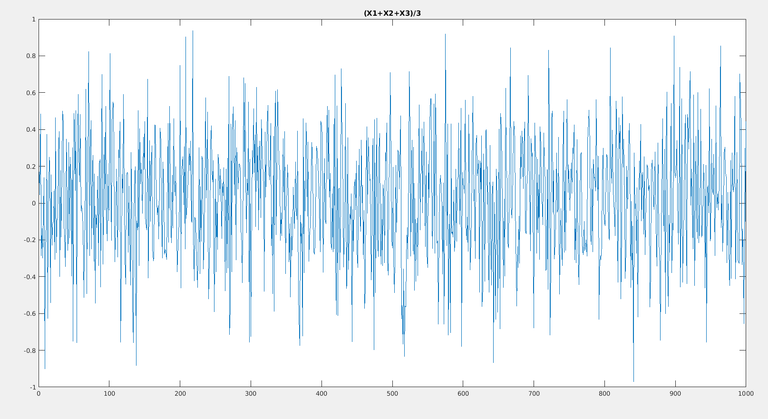
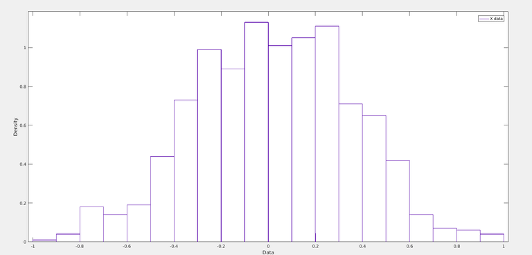
Let us repeat with (X1+X2+X3)/3 and its distribution :

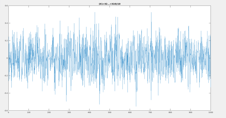
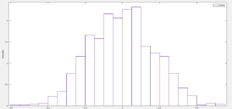
Let us repeat this say X1 to X10 now :

Distribution (N=10 case) :

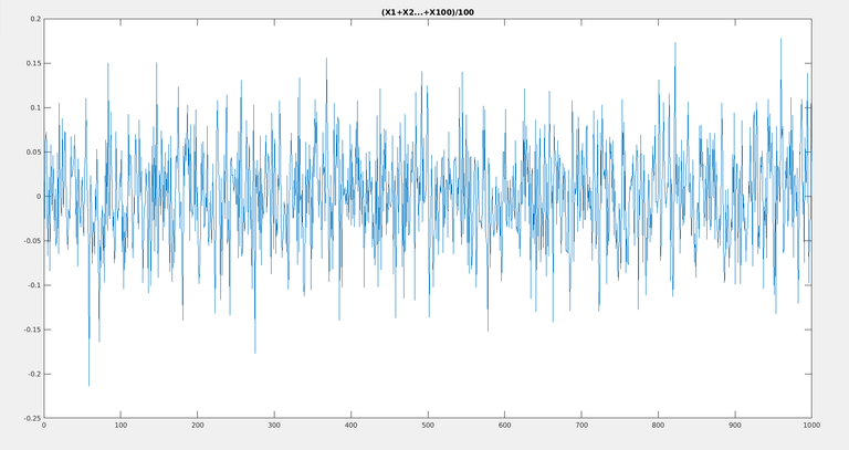
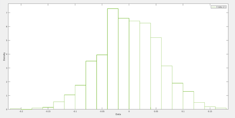
Let us see N=100 case next !

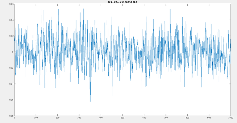
N=1000 :

And its density :

So what is really happening :

The distribution started as uniform flat one, next triangular one .. ultimately it will reach something like below :

![](

So what actually happens is that as you add random variables, their individual probability densities get "convolved" each time to generate equivalent density. If you convolve a flat distribution with another you get a triangle distribution. If you keep on repeating this infinitely you end up with ideal Normal distribution!

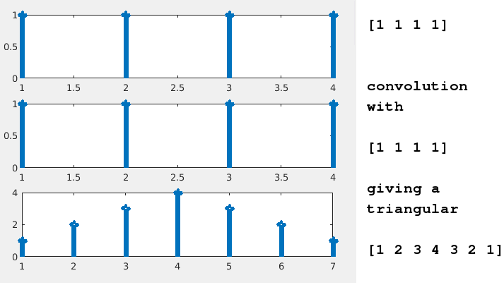
So what is convolution? For now please see this wiki link. For discrete sequences, I will give you a simple example here. If you wanted to convolve [1 1 1 1] and [1 1 1 1], the result will be like below:

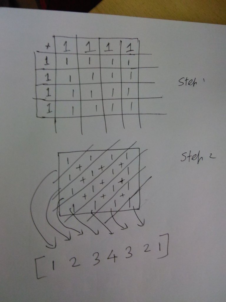
Convolution ([1 1 1 1], [1 1 1 1]) = [1 2 3 4 3 2 1]

If you continue this forever, you end up with the bell-shaped gaussian !

All the plots above are created in Matlab programming language.

Hi,
I am Devanand from Chennai, India. And my steemit handle is @dexterdev
Do you like my posts? Please do reply for your doubts etc. Also Resteem and Upvote if you like these posts!
If you would like to see any improvements, please tell me.
Also, Follow me! :)

Central Limit Theorem : Visually Explained!