In my previous articles, we have seen many examples which demonstrated classical molecular dynamics simulations of bigger systems like
- Protein complex in water box
- A lipid bilayer patch system in water box
- Protein interacting with lipid bilayer patch in water box
etc
Today let us attempt something very simple. Very less math(or math that you can ignore and still you can understand most of the stuff!) and more intuitive explanation will be the focus of today's article. (Although this is what I strive always for... Don't know how successful I am in doing so. Do let me know via comments.) Let us try to get an intuition from this toy system.
The System
Think about a system where you have a hypothetical particle in a crowd of lot many smaller particles(ideally in the order of 1023, but lesser number will also work, which can be considered a large number. Why this number? Let that be a homework now.) The situation will be something like as below:
Image Source: Wikimedia, Author: Lookang, Author of computer model: Francisco Esquembre, Fu-Kwun and lookang, License: CC BY-SA 3.0
The small particles will have an inherent random motion in them where they collide each other and with the bigger particle too. Now this bigger particle will also exhibit a random motion due to this. This is typically called Brownian motion(The name from an 1827 biologist Robert Brown who observed via microscope that pollen grains jiggle in water) which emerges as a result of random walks. The classical molecular dynamics which we were doing in the past was very deterministic. Here we see randomness. Why so? Is there some inconsistency? There is no inconsistency. The thing is if each of these particles was allowed to move according to newtons laws(where we also know their initial positions and velocities) would exhibit some dynamics like this. The thing is when we have a lot of such trajectories we can try to model this uncertainty using randomness or noise terms. And gaussian noise is a good model to achieve this.
So if you don't want to track all of these nasty small particles you can resort to something called Langevin Dynamics. This is different from Classical Molecular dynamics. In classical molecular dynamics: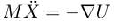
is the equation of motion. mass times acceleration is the force which is the negative gradient of potential energy U. We have explained these things before.
Now in the langevin formalism, the small particles become implicit. So the equation becomes:
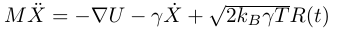
where the second term in the right hand side of the equation is gamma(friction coefficient) times velocity and the third term is the noise term. R(t) is a zero mean, delta correlated stationary gaussian noise and scaling factor  is where the temperature T comes in the picture. Intuitively we can assume that when the temperature is high the diffusion coefficient(D) of the bigger particle will be high and if the viscosity is high the diffusion coefficient of the larger particle will be lesser. There is a relation which Einstein derived in 1905 for this:
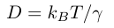
This is one of the earliest so called fluctuation-dissipation relation.
The potential decides what force the particle experiences. Now think about a double well potential like this below:
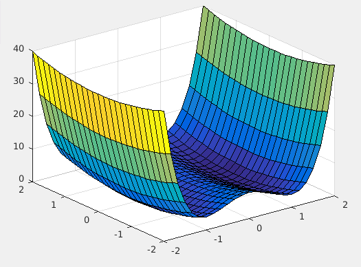
If you slice it in one dimension(at Y=0) you will see that it has 2 minimas: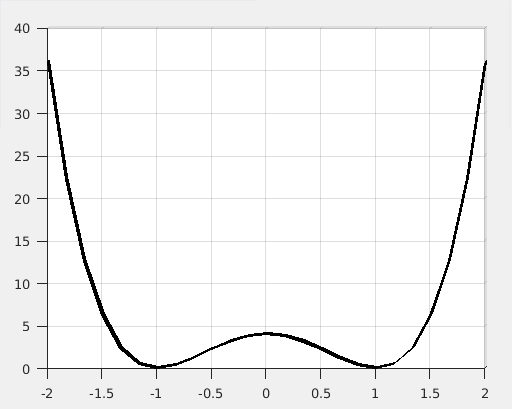
This is why we are calling it double well potential. The form of the potential energy function is as below:
where X and Y are particle position coordinates.
Matlab code for the plotting potential:
clear; close all; clc
x=linspace(-2,2,25);
y=linspace(-2,2,25);
[X,Y] = meshgrid(x,y);
Z=4*(X-1).^2.*(X+1).^2 + Y.^2; % potential energy landscape
hs = surf(X,Y,Z); % Get surface object
Now imagine that our particle which experiences friction and kicks(noise) from the other particles and is also under influence of this particular potential energy . Depending on the temperature T, friction coefficient gamma and the barrier height of the potential(the peak between minimas) our particle will traverse in this energy landscape. Let us see that dynamics via a very simple simulation which we can setup in openMM.
The implementation of system using openMM toolkit
OpenMM is a collection of python packages which help users to create python scripts to run MD simulations. It is a toolkit from Vijay Pande group which pioneered the folding@home project.
Python Code(Which I wrote on Jupyter notebook initially):
%matplotlib inline
from __future__ import print_function
import numpy as np
import matplotlib.pyplot as plt
import simtk.openmm as mm#Imported numpy, plotting libraries and openmm
def run_simulation(n_steps=10000):
"Simulate a single particle in the double well"
system = mm.System()
system.addParticle(1)# added particle with a unit mass
force = mm.CustomExternalForce('2*(x-1)^2*(x+1)^2 + y^2')# defines the potential
force.addParticle(0, [])
system.addForce(force)
integrator = mm.LangevinIntegrator(500, 1, 0.02)% Langevin integrator with 500K temperature, gamma=1, step size = 0.02
context = mm.Context(system, integrator)
context.setPositions([[0, 0, 0]])
context.setVelocitiesToTemperature(500)
x = np.zeros((n_steps, 3))
for i in range(n_steps):
x[i] = context.getState(getPositions=True).getPositions(asNumpy=True)._value
integrator.step(1)
return x
trajectory = run_simulation(25000)
ylabels = ['x', 'y']
for i in range(2):
plt.subplot(2, 1, i+1)
plt.plot(trajectory[:, i])
plt.ylabel(ylabels[i])
plt.xlabel('Simulation time')
plt.show()
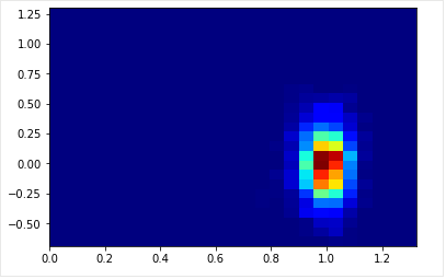
plt.hist2d(trajectory[:, 0], trajectory[:, 1], bins=(25, 25), cmap=plt.cm.jet)
plt.show()
Explanation of the code
What we are doing here is initiating a single particle which experiences the friction and kicks and evolves its positions via langevin integrator. system.addParticle(1) means adding a particle with unit mass, force = mm.CustomExternalForce('2*(x-1)^2*(x+1)^2 + y^2') is where you define the potential, integrator = mm.LangevinIntegrator(500, 1, 0.02) is where you define the bath temperature, gamma(friction coefficient=1) and step size(0.02). trajectory = run_simulation(25000) calls the simulation run for 25000 steps. and the rest is plotting step.
Results
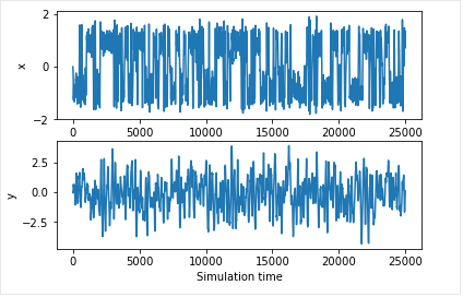
The double well is very visible from the positions of x. The particle moves back and forth between 2 wells.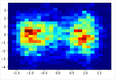
This is a histogram of x versus y coordinates. Again you can see that there are 2 valleys here.
Different cases
Let us think about a case where the temperature is very low. Let us put T=10K. The particle should not leave one minima, right? Let us see: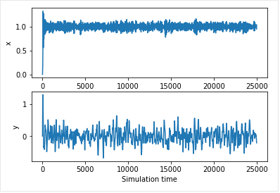
Indeed that is the case!
What should happen if we increase friction coefficient keeping T=500K? Let us put gamma=100.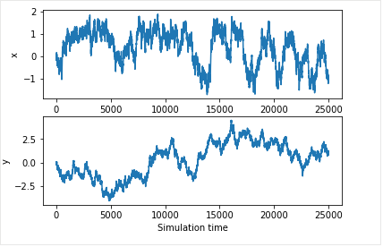
Of course, the transitions became lesser in frequency! The effect of higher viscosity!
Now, what happens if we raise the barrier of potential. This was the potential: If I change 4 to 20, the barrier between wells will rise. Which means the particle will find it hard to jump the barrier. Let us repeat the experiment by only changing this parameter from the original experiment: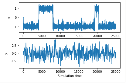
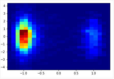
Indeed that is the case! So if you try to reconstruct energy landscape from the above case, it will give a biased profile. So one solution can be running the simulation longer. Let us try?
Instead of 25000 steps, let us run the simulation for 250000 steps.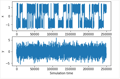
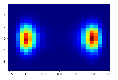
See the symmetric well is very visible now! If you reconstruct the energy surface from here it will be a good estimate.
Code Repository
All code available here:
https://github.com/dexterdev/STEEMIT/tree/master/Particle_in_double_well_potential
Installing the openMM python library
To install openMM, just do:conda install -c omnia -c conda-forge openmm
assuming you have installed anaconda python package in a 64 bit linux machine. For other cases and more details see instructions here.
References, links, and further reading
Some MD fundamentals:
- https://steemit.com/steemstem/@dexterdev/classical-molecular-dynamics-series-part-1-the-fundamentals
- https://steemit.com/steemstem/@dexterdev/classical-molecular-dynamics-series-part-2-the-force-field
- https://steemit.com/steemstem/@dexterdev/classical-molecular-dynamics-series-part-3-solving-the-molecular-dynamics-equation
A book reference: "Statistical Mechanics: Theory and Molecular Simulations" by Mark E. Tuckerman
#steemSTEM
#steemSTEM is a very vibrant community on top of STEEM blockchain for Science, Technology, Engineering and Mathematics (STEM). If you wish to support steemstem visit the links below:

Quick link for voting for the SteemSTEM Witness(@stem.witness)
Delegation links for @steemstem give ROI of 65% of curation rewards
(quick delegation links: 50SP | 100SP | 500SP | 1000SP | 5000SP | 10000SP).
Also, visit and create your STEM posts using steemstem app here: https://www.steemstem.io
You can also set @steemstem as beneficiary.

The animated title pic really does a fantastic job of drawing the viewer in. I'll have to try that at some point. Also, very cool introduction to Brownian motion and how coding can help analyze this phenomena.
This reminds me of a very simple atomic model I produced at school. That was many years ago and the computers were not up to what can be done now.
Wow, and I thought I worked hard on my posts :D
:P I have to improve a lot though.
I don't know if you have to, but everyone can and progress is in big part what life is about I think. :)
Oooo my God...... Interesting things there in your blog and for so many years I never really met most of the things in said in your blog, which simply means, am really educated today. And I enjoyed the class even though I didn't pay an tuition..... Lol
Lovely work in there and every time spent on your blog was really worth it. Great pictures too.
Great work and keep the science and technology spirit up
Posted using Partiko Android
😃
Cool
Posted using Partiko Android
Wow, very nice. But I have to admit I have to read your other publications as well to get further into this subject. Where are these two minima from again? Don't get it!
Regards
Chapper
Hi @chappertron : Thank you for stopping by :) So the minimas are embedded in the potential function which I defined in the beginning.
This is how the function is:
You can see that there are 2 minimas at X=1 and X=-1 in this function.
See this plot(@ Y=0):

You saw the 2 minimas? Our particle toggles between these 2 states.
Oh of course! I have to look closer next time. Reminds me of my biophysics courses at the University used to.
So this equation would explain why the yellow dot moves as it moves in a crowd of smaller particles?
No. If the yellow particle was allowed to move freely, Potential surface would be like a flat plane surface. But now if I compel my particle under this curvy potential with two minimas, that is what I am defining by this equation. Great question btw. I should have been more clear in the article. But I hope people read comment section too. :)
By the way, just defining this potential function won't make things alive. That's what the langevin equation is there. That equation gives life to the particle under whatever potential you define.
Very cool reply!
The langevin equation makes things become alive
That's mathematics at it's best.
Thanks again
Best
Chapper
This post has been voted on by the SteemSTEM curation team and voting trail. It is elligible for support from @curie and @utopian-io.
If you appreciate the work we are doing, then consider supporting our witness stem.witness. Additional witness support to the curie witness and utopian-io witness would be appreciated as well.
For additional information please join us on the SteemSTEM discord and to get to know the rest of the community!
Thanks for having added @steemstem as a beneficiary to your post. This granted you a stronger support from SteemSTEM.
Thanks for having used the steemstem.io app. You got a stronger support!
Hi @dexterdev!
Your post was upvoted by Utopian.io in cooperation with @steemstem - supporting knowledge, innovation and technological advancement on the Steem Blockchain.
Contribute to Open Source with utopian.io
Learn how to contribute on our website and join the new open source economy.
Want to chat? Join the Utopian Community on Discord https://discord.gg/h52nFrV
The animated title pic really does a fantastic job of drawing the viewer in. I'll have to try that at some point. Also, very cool introduction to Brownian motion and how coding can help analyze this phenomena.
Congratulations! This post has been upvoted from the communal account, @minnowsupport, by dexterdev from the Minnow Support Project. It's a witness project run by aggroed, ausbitbank, teamsteem, someguy123, neoxian, followbtcnews, and netuoso. The goal is to help Steemit grow by supporting Minnows. Please find us at the Peace, Abundance, and Liberty Network (PALnet) Discord Channel. It's a completely public and open space to all members of the Steemit community who voluntarily choose to be there.
If you would like to delegate to the Minnow Support Project you can do so by clicking on the following links: 50SP, 100SP, 250SP, 500SP, 1000SP, 5000SP.
Be sure to leave at least 50SP undelegated on your account.
Congratulations @dexterdev! You have completed the following achievement on the Steem blockchain and have been rewarded with new badge(s) :
You can view your badges on your Steem Board and compare to others on the Steem Ranking
If you no longer want to receive notifications, reply to this comment with the word
STOPDo not miss the last post from @steemitboard:
Vote for @Steemitboard as a witness to get one more award and increased upvotes!