This is the fifth part of a 9 part tutorial series about the R Statistical Programming Language, targeted at data analysts and programmers that are active on Steem.
In this course you will learn the R programming language through practical examples.
![]()
Repository
The R source code can be found via one of the official mirrors at
This tutorial is part of a series, the text as well as the code is available in my github repo
What Will I Learn?
The first two tutorials introduced the basics of R and the free R Studio IDE, the rest of this series will focus on worked examples where we will slowly introduce new concepts and learn some of the extended functionality of the R programming language.
In this tutorial we will cover:
- Working with Time Series Data in R
- Download and Clean Data from the Web (Already covered in Previous Tutorials)
- Visualise the Time Series Data using Specialist R Packages
- Make Price Forecasts using an R Statistical Library
- Examine Diagnostic Plots for Time Series Data
Requirements
- Lesson 1 Introduction to R
- Lesson 2 Finding Your Way Around R
- Basic Knowledge of Statistics
- Basic Knowledge of Time Series
- Basic Programming Experience
- Some Knowledge of Steem and Cryptocurrencies
Difficulty
Intermediate

Time SeRies with R.
R provides rich data structures which allow you you to define structured embedded data objects. This enables intuitive data manipulation, analysis and modelling. Today we will learn more about R by exploring a few packages for working with time series data.
Time Series
A time series is a series of data points indexed in time. Most often this term is used to refer to the prices of some commodity over time, for example at daily intervals.
The basic time series object in R is called “ts”. We will look at more advanced time series in a few minutes but first we will look at the basic implementation in R. If you have a list of prices stored in a variable you can create a time series by typing the ts command.
We need some dummy data so lets create 10 random number sin R which we will call prices. In the console type
prices <- rnorm(10)
- The rnorm function creates an observation from the standard normal distribution. The argument 10 says create 10 of these. Each time you run this command you will get different random variables from the Standard Normal Distribution.
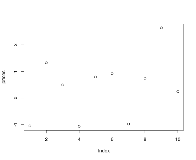
We can plot the Prices with the following command. You will get a graph similar to the following
plot(prices)
We will next create an R time series variable using this "dummy" price data. In the console type
ts.prices <- ts(prices)
- We passed our variable to the ts function
Plotting this variable
plot(ts.prices)
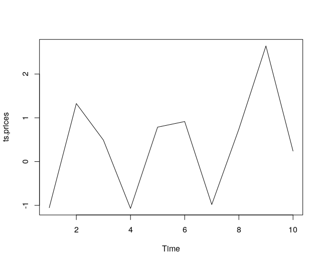
- Notice the points are now joined and the x axis is called Time.
Examine the ts.prices variable
ts.prices
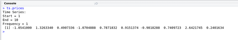
- We can see that our ts.prices data now has added structure. This is a basic time series in R.
We can now go into more detail and we will next look at some packages that extend the functionality of this basic time series object
Time Series Packages
In previous tutorials we have covered searching, installing and loading packages in R. We will load the following three packages which we will use in this tutorial:
XTS Package
This package provides a framework that aids integration of other time series packages but it also provides some helper functions such as data filtering. We will see an example of this where we can filter the data by year and month.
Install and load the package
install.packages(“xts”, dependencies=T)
library(xts)
Quantmod Package
This package is described as
designed to assist the quantitative trader in the development, testing, and deployment of statistically based trading model
In this tutorial we will not use the advanced functionality but we will use some of the Charting Functionality that has been included in this package.
Install and load the package
install.packages(“quantmod”, dependencies=T)
library(quantmod)
Forecast Package
This is a really useful package that provides tools for forecasting and analysing time series data.
Install and load the package
install.packages(“forecast”, dependencies=T)
library(forecast)
Download & Clean Steem Price Data
In previous tutorials we went into detail about downloading and cleaning data. We will use some of those techniques here to get historical data about the Steem Price and clean it.
If you need a refresher on the basics you can review those previous tutorials
Get historical CMC data for Steem
library(htmltab)
url <- "https://coinmarketcap.com/currencies/steem/historical-data/?start=20160701&end=20180813"
cmc <- htmltab(url)
Clean the data
Convert to a data.table
cmc <- data.table(cmc)
Select the Columns to Keep
cmc <- cmc[, c("Date", "Volume", "Open", "High", "Close*", "Low")]
Rename the Columns
names(cmc) <- c("Date","Volume","Open","High","Close", "Low")
Convert the data to numeric format (from Strings)
cmc[, Open:=as.numeric(Open)][, High:=as.numeric(High)][, Low:=as.numeric(Low)][, Close:=as.numeric(Close)]
cmc[, Volume:=as.numeric(gsub(",","",Volume))]
Convert the dates to date format (from Strings)
cmc[,Date:=as.Date(Date, "%b %d, %Y")]
After you have ran these commands typing cmc in the console should show the following dataset
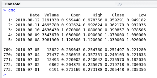
- We have now downloaded our data, cleaned it and stored it in a rectangular data structure. We are ready to use some of the more advanced packages to see what R can do with time series data.
Using the XTS Library
convert the data to an XTS object
library(xts)
cmc.xts <- as.xts(cmc)
We will take a quick look at our data in the console. Type cmc.xts
cmc.xts
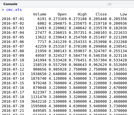
- You can see the data is now structured as a time series and shows the date and price at each date.
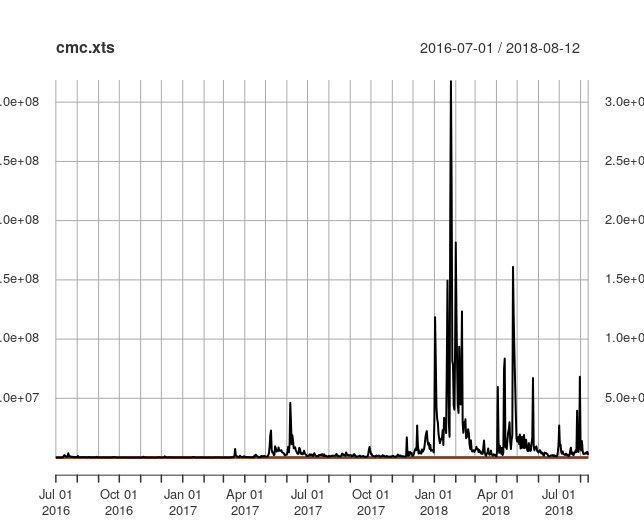
We can plot the data with the following command
plot(cmc.xts)
Advanced Visualisations
Data cleaning is usually a slow laborious process but we can see that we now have a script with just a few lines of code that can be modified and updated regularly. Once we have built our data structure we can leverage add on R packages to meet our needs. We will now plot some candle charts of the Steem price using the quantmod package.
library(quantmod)
candleChart(cmc.xts)
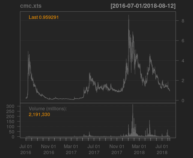
- This shows a really nice visualisation of the Price over time.
What if we wanted just wanted observations in 2018? We can pass a year value to the xts variable.
candleChart(cmc.xts["2018"])
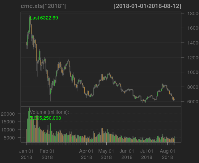
- Not a pretty picture!
To display observations for August
candleChart(cmc.xts["2018-08"])
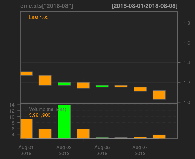
- Using the interactive console it is really easy to modify formulas and try out variations until you get what your looking for.
Exercise
I will leave it up to you to run this same analysis to get the Bitcoin Price and plot a candle chart for August.
- It should look like the following graph.
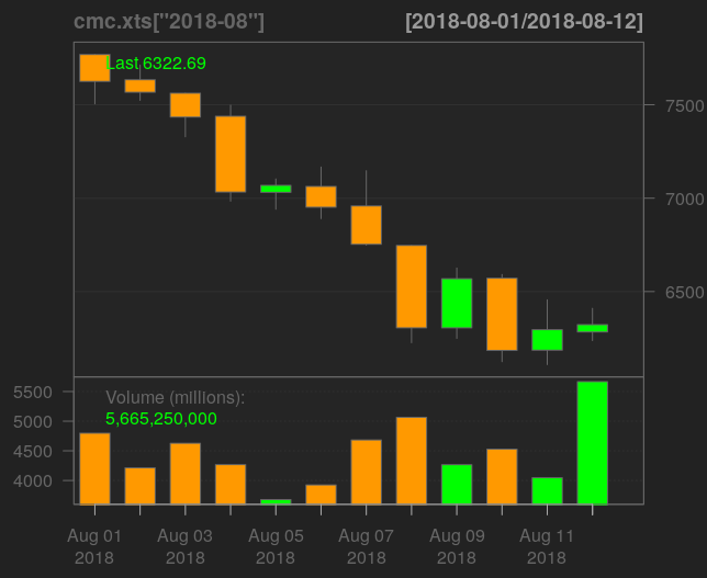
- A script with the solutions can be found at my github to reproduce the above chart.
Forecasting
This tutorial does not aim to provide the science behind technical forecasting but we introduce the R forecast package which includes all manner of time series forecasting tools and diagnostics.
The closing Steem price can be retrieved from our xts object by indicating the column name. We will save this as a variable called close.price
close.price <- cmc.xts$Close
To forecast the closing price we just need to type
forecast(close.price)
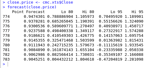
- This defaults to give 10 forecast values and confidence intervals around the point estimates.
- The default prediction model use is “Exponential smoothing state space model” but can be customised in the paramaters. For a full list of available paramaters you can explore the package documentation in more detail with the command help(“forecast”)
Diagnostics
Accurate Time Series modelling relies on data having certain statistical properties such as being stationary. R provides tools to examine the properties of time series data.
For example, we can examine if a series is differencing stationary by looking at the difference of the daily price values
close.price
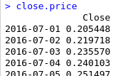
- This prints the daily prices
Using the diff function we can get the difference
diff(close.price)
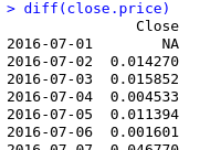
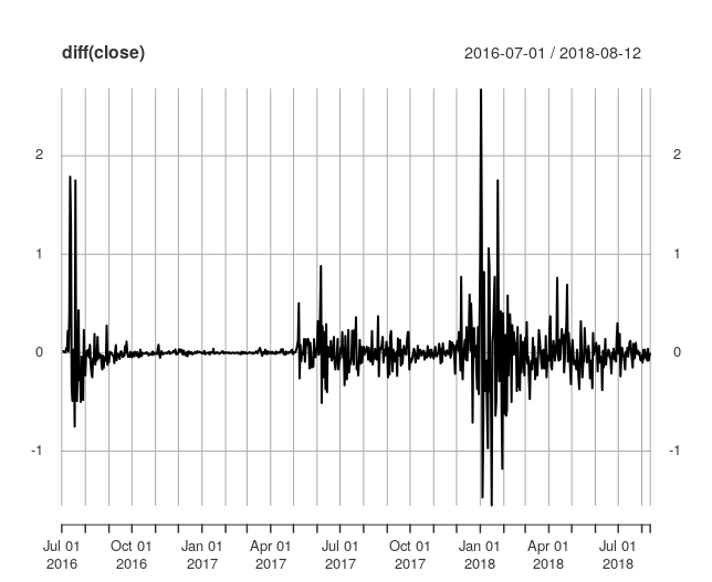
If the data is differencing stationary we should see difference values centered around 0
plot(diff(close.price))
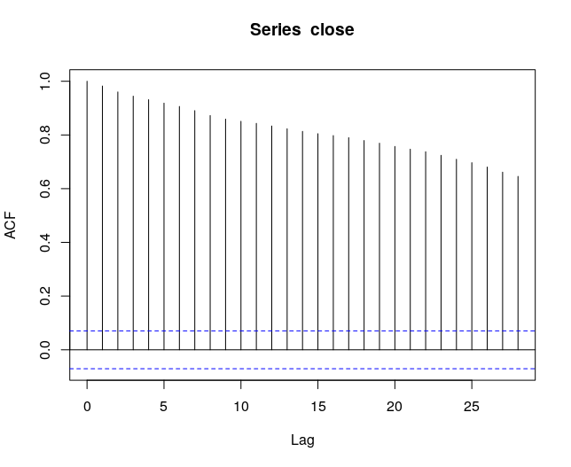
We can also examine autocorrelation which is another statistical property using the acf function
plot(acf(close.price))
Recap
In this lesson we covered:
- Working with Time Series Data in R
- Download and Clean Data from the Web (Already covered in Previous Tutorials)
- Visualise the Time Series Data using Specialist R Packages
- Make Price Forecasts using an R Statistical Library
- Examine Diagnostic Plots for Time Series Data
Benefits of Using R for Time Series
- Visualisation
- Time Series Data Manipulation
- Advanced Modelling and Diagnostic tools
Code Used
Illustrate a Time Series object
Generate and plot 10 observations from a Random Normal Distribution.
prices <- rnorm(10)
plot(prices)
##Convert the Variable prices to a time series object
ts.prices <- ts(prices)
plot(ts.prices)Get & Clean Steem Price data from coinmarket cap
Download the Prices
library(htmltab)
url <- "https://coinmarketcap.com/currencies/steem/historical-data/?start=20160701&end=20180813"
cmc <- htmltab(url)Clean the data
cmc <- data.table(cmc)
##Subset the Columns
cmc <- cmc[, c("Date", "Volume", "Open", "High", "Close*", "Low")]
##Rename the columns
names(cmc) <- c("Date","Volume","Open","High","Close", "Low")
##Convert the Data
cmc[, Open:=as.numeric(Open)][, High:=as.numeric(High)][, Low:=as.numeric(Low)][, Close:=as.numeric(Close)]
cmc[,Date:=as.Date(Date, "%b %d, %Y")]
cmc[, Volume:=as.numeric(gsub(",","",Volume))]
library(xts)
cmc.xts <- as.xts(cmc)
plot(cmc.xts)
##Use Quantmod to Plot the Data
library(quantmod)
candleChart(cmc.xts)
candleChart(cmc.xts["2018"])
candleChart(cmc.xts["2018-08"])
##Forecast the data
library(forecast)
close.price <- cmc.xts$Close
forecast(close.price)
##Analyse the Data for Stationarity and Autocorrelation
close.price
diff(close.price)
plot(diff(close.price))
plot(acf(close.price))
Coming up
This course will cover the basics of R over a series of 9 lessons. We began with some essential techniques (in the first 2 lessons) and I will take you on a tour of some of the more advanced features of R with worked examples that have a Cryptocurrency and Steem flavour.
My favourite feature of R is the advanced visualisations and plotting capabilities. We have already seen some of the capabilities of R but we will go into more detail in the next lesson on powerful features such as faceting and give an introduction to the implementation of the Grammar of Graphics in R.
Curriculum
For a complete list of the lessons in this course you can find them on github. Feel free to reuse these tutorials but if you like what you see please don't forget to star me on github and upvote this post.
Related Posts
- Lesson 1 Introduction to R
- Lesson 2 Finding Your Way Around R
- Lesson 3 Scraping Web Data with R
- Lesson 4 Data Wrangling with R
Thank you for reading. I write on Steemit about Blockchain, Cryptocurrency and Travel.
R logo source: https://www.r-project.org/logo/
Thank you for your contribution.
Looking forward to your upcoming tutorials.
Your contribution has been evaluated according to Utopian policies and guidelines, as well as a predefined set of questions pertaining to the category.
To view those questions and the relevant answers related to your post, click here.
Need help? Write a ticket on https://support.utopian.io/.
Chat with us on Discord.
[utopian-moderator]
Thank you for your review, @portugalcoin!
So far this week you've reviewed 13 contributions. Keep up the good work!
Congratulations! Your post has been selected as a daily Steemit truffle! It is listed on rank 17 of all contributions awarded today. You can find the TOP DAILY TRUFFLE PICKS HERE.
I upvoted your contribution because to my mind your post is at least 14 SBD worth and should receive 93 votes. It's now up to the lovely Steemit community to make this come true.
I am
TrufflePig, an Artificial Intelligence Bot that helps minnows and content curators using Machine Learning. If you are curious how I select content, you can find an explanation here!Have a nice day and sincerely yours,

TrufflePigHey @eroche
Thanks for contributing on Utopian.
Congratulations! Your contribution was Staff Picked to receive a maximum vote for the tutorials category on Utopian for being of significant value to the project and the open source community.
We’re already looking forward to your next contribution!
Want to chat? Join us on Discord https://discord.gg/h52nFrV.
Vote for Utopian Witness!
Thanks u for sharng this