In this video I go over an example on the Lotka-Volterra predator-prey equations to see how to solutions are graphically estimated. This example involves graphing solutions on a direction field based on the Predator-Prey plane, as opposed to the typical function and time axes. I go over parts a), b), and c) of this example, and I will go over the rest of the example in my next video on Part 2, so stay tuned for that! This is a great example to see how differential equations can be used to model two different species populations and how to interpret the resulting solutions.
Watch on DTube:
Watch on BitChute: https://www.bitchute.com/video/WXQTYteWKY7E/
Download PDF Notes: https://1drv.ms/b/s!As32ynv0LoaIht0mB0v6c2t3Hr5OFQ
View Video Notes Below!
Download These Notes: Link is in Video Description.
View These Notes as an Article: https://steemit.com/@mes
Subscribe via Email: http://mes.fm/subscribe
Donate! :) https://mes.fm/donateReuse of My Videos:
- Feel free to make use of / re-upload / monetize my videos as long as you provide a link to the original video.
Fight Back Against Censorship:
- Bookmark sites/channels/accounts and check periodically
- Remember to always archive website pages in case they get deleted/changed.
Join my private Discord Chat Room: https://mes.fm/chatroom
Check out my Reddit and Voat Math Forums:
Buy "Where Did The Towers Go?" by Dr. Judy Wood: https://mes.fm/judywoodbook
Watch my #AntiGravity Video Series: https://mes.fm/antigravity-playlist
Follow My #FreeEnergy Video Series: https://mes.fm/freeenergy-playlist
NOTE: If you don't have time to watch this whole video:
- Play this video at a faster speed.
--TOP SECRET LIFE HACK: Your brain gets used to faster speed. (#Try2xSpeed)
--Try 4X+ Speed by Browser Extensions, HookTube.com, Modifying Source Code.
--Browser Extension Recommendation: https://mes.fm/videospeed-extension- Download and Read Notes.
- Read notes on Steemit #GetOnSteem
- Watch the video in parts.
Example:
Suppose that populations of rabbits and wolves are described by the Lotka-Volterra equations (https://youtu.be/b3NCjsZhQdQ) with k = 0.08, a = 0.001, r = 0.02, and b = 0.00002.
Assume the time t is measured in months.
a) Find the constant solutions (called the equilibrium solutions) and interpret the answer.
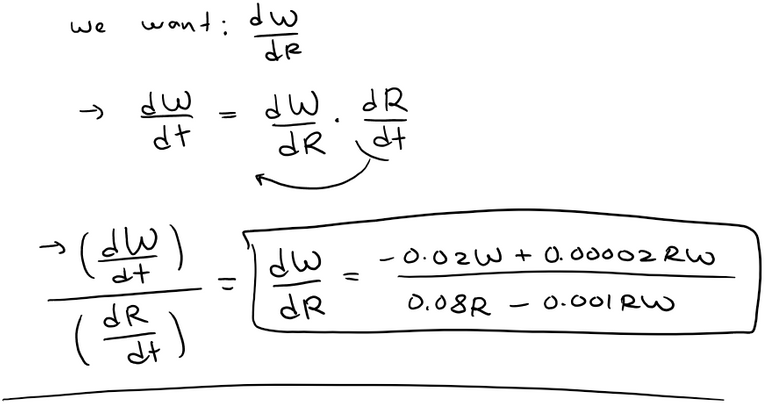
b) Use the system of differential equations to find an expression for dW/dR.
c) Draw a direction field for the resulting differential equation in the RW-plane.
Then use that direction field to sketch some solution curves.
d) Suppose that, at some point in time, there are 1000 rabbits and 40 wolves.
Draw the corresponding solution curve and use it to describe the changes in both population levels.
e) Use part (d) to make sketches of R and W as functions of t.
Solution

a) Both R and W will be constant if both derivatives are 0, i.e. populations are not growing or decreasing.
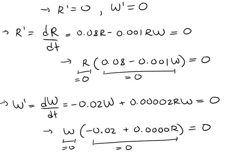
A trivial solution is given by R = 0 and W = 0.
- This makes sense: If there are no rabbits or wolves, the populations are certainly not going to increase.
The other constant solution is:
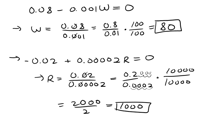
So the equilibrium populations consist of 80 wolves and 1000 rabbits.
This means that 1000 rabbits are just enough to support a constant wolf population of 80.
There are neither too many wolves (which would result in fewer rabbits) nor too few wolves (which would result in more rabbits).
b) We can use the Chain Rule:

Notice that the curves appear to be closed in the sense that if we travel along a curve, we always return to the same point.
Notice also that the point (1000, 80) is inside all the solution curves.
That point is called the equilibrium point because it corresponds to the equilibrium solution:
R = 1000, W = 80
When we represent solutions of a system of differential equations as in the direction field above, we refer to the RW-plane as the phase plane, and we call the solutions curves phase trajectories.
So a phase trajectory is a path traced out by solutions (R, W) as time goes by.
A phase portrait consists of equilibrium points and typical phase trajectories.