Hello friends... Welcome to my new molecular dynamics post. As I mentioned in my previous post, I am going to start the new series on coarse-grained lipid models. As an opening article to this series, I will start with a toy example which will make you familiarize with the software LAMMPS, tools topotools, and VMD etc. I have mentioned about VMD in previous article series on MD:
Part 1 (The Fundamentals)
Part 2 (The Force Field!)
Part 3 (Solving the molecular dynamics equation)
Part 4a (Setting up NAMD simulation and running it)
Part 4b (Running small systems on your computer)
Today we are going to try a system which will exhibit aggregation of molecules:
(Aggregation of molecules simulated via LAMMPS)
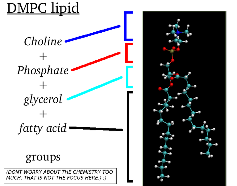
My previous articles were about all-atom molecular dynamics simulations. This means that we care about each individual atoms. Even hydrogen atoms matter. The partial charges and mass of every atoms whether it be carbon atom or nitrogen atom. Every detail matter. In contrast to this, what I am going to talk from today is something called coarse-grained molecular dynamics. We dont simulate "atoms" here. But you simulate particles that will "hopefully" capture the global dynamics of systems. (But it is a common practice to call atom and particle interchangeably). Remember our DMPC lipid molecule? See the figure below:
(Image Courtesy: @dexterdev)
This lipid molecule has phosphocholine head(which is hydrophilic, i.e water liking group) and fatty acid tails(hydrophobic or water hating). What if a Physicist who loves spherical cow models wanted to just study about certain phenomenon of lipids. One way to proceed is to come up with hypothetical models for lipids. Like as in below:
This is a 3 bead lipid model where 1st particle is hydrophilic and other two particles are hydrophobic!(Image Courtesy: @dexterdev)
Outrageous, right? How can these physicists remove the entire details. Of course biologists will not be happy! But surprisingly enough there are many features which these models can capture. Not just that it makes modelling them in computer easy. Larger systems can be simulated for long enough without having too much of computing luxury.
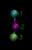
Let us get into the business right now. My aim is to illustrate the phenomenon of aggregation using a minimal coarse-grained model using LAMMPS. For that purpose I will define a 2 bead particle.
Two bead(type 1 and type 2) particle(Image Courtesy: @dexterdev)
Bonding between particles
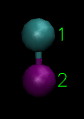
At this point it is very important to understand what kinds of interactions we define between particles. There are kind of interactions which I will explain in this example. First kind of interaction is between the particles in a single "molecule". For example, between particles 1 and 2 in the two bead particle. This is to mimick a covalent bond, which can be realized by a harmonic spring. Please see this article to understand covalent bonds better: Article on harmonic oscillators, Hookes law and bonded interactions.
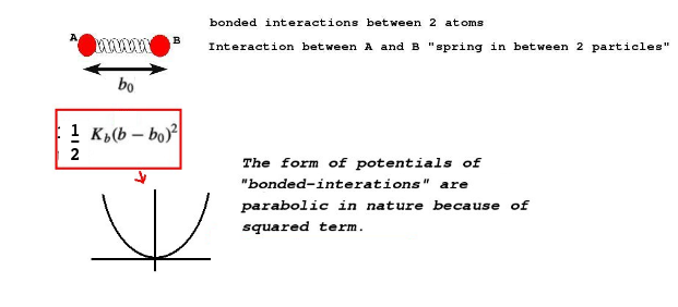
b_0 is the equilibrium bondlength, K_b is the bond coefficient. Higher the bond coefficient higher will be the stiffness of the bond.(Image Courtesy: Adapted from my previous article on force fields)
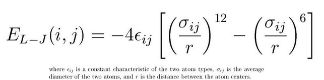
The second type of interaction is to mimick the non-bonded interactions in the form of Lennard-Jones potential. Also known as LJ potential actually approximate the interactions between neutral atoms. LJ potential has a mathematical form as below:
(Image Courtesy: Adapted from my previous article on force fields)
The (1/r)^12 is the repulsion term and the (1/r)^6 term is the long-range attraction term. Higher epsilon term in the LJ potential means the minima in the potential term is deeper. That means the attraction will be higher between LJ particles. Usually we assign a cut-off at 2.5 sigma so as to not compute the interactions till infinity. Once you cutoff at this value, you have to make the function smooth by adding higher differentials appropriately or clamp(shift) the entire potential to zero potential. The LJ potential looks like below:
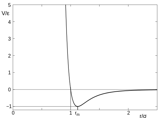
(Image Courtesy: wikimedia, Image by Olaf Lenz, manually modifield by Rainald62, License: CC BY-SA 3.0)
The third potential necessary for today's example is something called WCA(Weeks-Chandler-Andersen) potential, which is just the repulsion term till r_m in LJ(and no attraction term), but clamped(shifted) to zero potential. The particles just gets repelled if they interact via WCA potential.
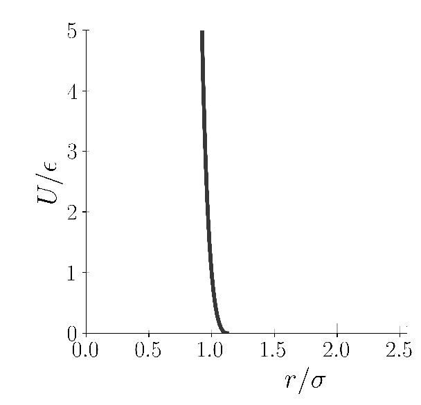
WCA potential(Image Courtesy: @dexterdev)
Modelling the system using LAMMPS
Setting up the system
As mentioned before we will simulate a 2 particle "molecule", but 500 of them. The initial system looks like this. (This is a bunch of molecules from a failed simulation. :P So I got randomly placed 500 molecules.)
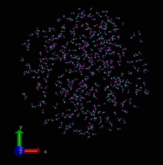
System of 500 hypothetical 2 bead molecules visualized in VMD software. (Image Courtesy: @dexterdev)
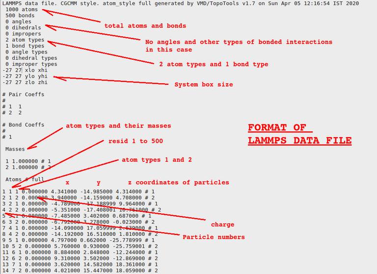
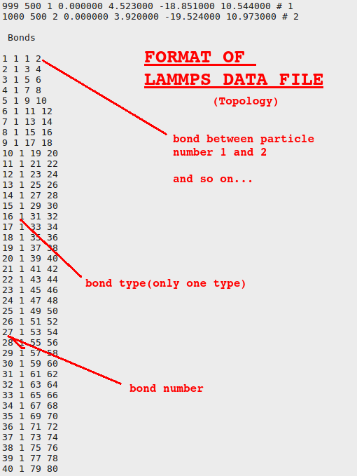
Our topology plus initial coordinate file: https://github.com/dexterdev/Molecular_Dynamics/blob/master/AGGREGATION_EXAMPLE/2p_mol.data
Topology means how particles in a molecule is connected and coordinates are the x, y, and z coordinates of different particles. Let us see how they look like inside the file:
.
.
.
.
LAMMPS scripts:
- system.in.settings
    pair_coeff  1 1   10.0  1.0  2.5
    pair_coeff  2 2   1.0  1.0  2.5
    pair_coeff  1 2   1.0  1.0  1.122
    bond_coeff  1   300.0 1.0
What this means is that between type 1 and 1 atoms(from different molecules), the epsilon of LJ potential is (10.0) and comparing to between 2 and 2 interactions(1.0), the minima is 10 times deeper and so 1 and 1 attracts each other strongly than between 2 and 2! 2.5 represents the sigma where cutoff is done. Now coming 3rd line it defines the interaction between type 1 particle of one molecule with type 2 of others. This is a WCA potential. Only repulsion exists. Because the cutoff happens at 1.122. Actually you have to shift the potentials to zero. That is done in next script. That was pair_coeff commands. Now comes the bond_coeff, which defines the harmonic interaction for type 1 and 2 atoms in the same molecule. Its bond_coefficient is 300.0 and the equillibrium bond distance is 1.0. A note about units. This is all in reduced LJ units. So the units are all in dimensionless forms.
- system.in.init
    dimension 3
    boundary        p p p
    units           lj
    atom_style      full

    bond_style      harmonic
    pair_style  lj/cut 2.5
    pair_modify shift yes

    neigh_modify    every 1 delay 1
    neighbor        0.3 bin
This script defines the 3D nature of simulation via dimension 3. boundary p p p means periodic boundary condition is 3 dimensions. We mentioned about units in the previous paragraph. atom_Style full is easy to understand and so I recommend you to go their documentation. bond_style is defined as harmonic as mentioned before. Other options like FENE do exist. But we will discuss it another point of time. the lj/cut at 2.5 and shifting to 0 potential was mentioned in last paragraph. While computing the program calculates a neighbor list. if we specify 0.3 bin as neighbor it takes neighbor molecules into a list from that total cutoff + 0.3 sigma distance and then compute LJ interactions among those. neigh_modify modifies list every steps you feed. In this case it calculates every step and updates the neighbors.
- minimization.in
# -- Init section --

include system.in.init

# -- Atom definition section --

read_data 2p_mol.data

# -- Settings Section --

include system.in.settings

# -- Run section --

dump            1 all custom 500 2p_mol_min.lammpstrj id mol type x y z ix iy iz
thermo_style    custom step pe etotal vol epair ebond eangle
thermo          20  # time interval for printing out "thermo" data

min_style quickmin
min_modify dmax 0.3


neigh_modify every 1 delay 0 check yes

minimize 1.0e-7 1.0e-9 10000 300000


write_data  2p_mol_after_min.data
This script minimizes the structure/topology file 2p_mol.data and spits out the minimization trajectory file and final minimized 2p_mol_after_minimization.data file. If you look into the file you will see that we loaded 3 files. 2 settings scripts and the 2p_mol.data coordinate/topology data file. Now this script will check for steric clashes or hinderances and try to achieve a local minima for the system.
You can run it using the command lmp_serial < minimization.in > min.log on your computer. Once the minimized structure is available, you can feed it for the simulation run.
- simulation run script
run_nvt.in
# -- Init Section --

include system.in.init

# -- Atom Definition Section --

read_data 2p_mol_after_min.data

# -- Settings Section --

include system.in.settings

# -- Run Section --


timestep      0.01
dump          1 all custom 10 2p_mol_nvt_.lammpstrj id mol type x y z ix iy iz


thermo_style  custom step temp pe etotal vol epair ebond eangle
thermo        100  # time interval for printing out "thermo" data

fix 1 all langevin 0.9 0.9 1.2 48279
fix 2 all nve


run           100000
write_data 2p_mol_nvt_.data
We again loaded 3 files. The settings scripts and the minimized structure. Then we are defining the step size of 0.01. dump is a command which will dump coordinates and other information to the trajectory file. thermo will spit out the time step, temperature, potential energy, total energy etc...
fix 2 all nve defines the classical molecular dynamics velocity verlet integrator. But if you ensembles other than NVE ones like NVT, you need a thermostat to be coupled with the system. In this example we use langevin thermostat(fix 1 all langevin 0.9 0.9 1.2 48279) with temperature 0.9 epsilon. and 1.2 is the damping factor. and the number after that 48279 is a random seed. So the trajectory output 2p_mol_nvt_.lammpstrj looks like this:
(Aggregation of molecules simulated via LAMMPS)
Conclusion
The aggregation of the molecules can be attributed to the preferential interaction between type 1 atoms compared to that of 1-2 and 2-2 interactions.
So that is for today. Let me know your response via comments. Thank you. :)
Repository of the project:
https://github.com/dexterdev/Molecular_Dynamics/tree/master/AGGREGATION_EXAMPLE
What experiments will you do to test your model?
This was supposed to be a toy model. The formation of micelles and bicelles like structures are an expected outcome of this model. Now what we can do more is to see the dependency of temperature on these structures.
Do you have any specific suggestions?
I was just having trouble figuring out what the model was intended to predict and how you do measurements to test the prediction.
The model was intended to capture the phenomenon of aggregation. It arises from the fact that the type 1 particles interact strongly via deeper epsilon in their LJ potential comparing to other interactions. You can run this simulation longer and analyze the aggregation numerically.
I have never really taken the time to leave you a comment here. And god knows I have read that post again and again, as I used it to debug the markdown converter of the stem.openhive platform...
I would like to state that I have really appreciated this post. It is very clear and it actually triggers (even in someone like me) the will to try out the software to see how it works in details. However, my time is so limited I will never have the time to do that... sorry... I hope others may be more courageous.
And of course I am looking forward to the next episode of the series!
My MD fundamentals are shaky. The governing equations are Hamiltonian? Are dimension reduction tricks used to speed up the process?
Hello @mathowl : The governing equations are from classical mechanics (Newton's 2nd law) and so you can write it in terms of Hamiltonian. Making the equations dimensionless has few advantages:
I think you are confusing reducing dimensions with making dimensionless :P
With dimension reduction I mean: If you have an N-dimensional system (for example with states in \mathbb{R}^N ) then there could be symmetries present which allow you to move the system to an M-dimensional system with M < N. This is a useful trick in the study of Hamiltonian systems.
Hi @mathowl : Sorry for the confusion. Okay so coarse-grained simulations are indeed "dimensionally reduced" versions of original systems. Yes, a real lipid will access more configurations, but our 3 particle coarse-grained models will not have high frequency - low energy motions. Those motions are filtered out effectively. But still you can study many important phenomena. Also speed up certainly!
But is it possible to reduce the dimension of the coarse-grained simulation using symmetries in the governing equations?
You asking about reducing the dimension of already dimensionally reduced coarse grained system? I think we will lose lot of information then. But I don't know if there will be any symmetry existing in the system. It might depend on specific systems I guess. Maybe we can discuss on it if I am understanding your query in a wrong way.
If there is a symmetry or some conserved quantity then you can reduce the system without losing any of the dynamics. I am not sure if that is the case for your set of equations. We can discuss it at a later time :o)
If you appreciate the work we are doing, then consider supporting our witness @stem.witness. Additional witness support to the curie witness would be appreciated as well.
For additional information please join us on the SteemSTEM discord and to get to know the rest of the community!
Please consider using the stem.openhive.network app and including @steemstem as a beneficiary of this post. This could yield a stronger support.