머신러닝 라이브러리에 텐서플로우만 있느 것이 아니다. 또 하나의 강력한 툴로 알려진 scikit-learn 라이브러리를 사용하여 머신러닝을 해보자.
sklearn에서 Iris flower data set을 읽어 들이자. 이 부분은 텐서플로우 홈페이지에 예제 문제로서 다루고 있는 잘 알려진 예제이기도 하다. 아울러 메트릭스를 편리하게 다룰 수 있도록 numpy 라이브러리를 함께 불러들인다.
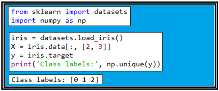
4개의 feature 컬럼 데이타들로 구성되는 Iris flower data set을 불러들인 후 그 중에서 3번째와 4번째 컬럼에 해당하는 [2, 3] 으로 표시되고 있는 꽃잎의 길이와 폭 데이터를 읽어 들이자. 그 다음은 읽어 들인 target의 라벨 값이 무엇인지 알아보기 위해서 np.unique(y)를 출력해 보자. 그 결과 라벨 값은 0, 1, 2 이며 즉 setosa, versicolor, verginica를 뜻한다.
train_test_split 라이브러리는 3종류의 붓꽃 데이터 각각이 50개씩인 150개의 샘플들로 이루어진 Iris flowers data set에서 학습용 데이터와 테스트용 데이터를 random하게 나누어 주는 역할을 한다. test_size 가 0.3 이라는 것은 70%를 학습용으로 그 나머지 30% 데이터는 테스트용으로 둔다는 것이며 random_state 값 지정은 반복 연산 시에 동일한 결과를 얻어 볼 수 있게 한다. stratify=y 는 특히 라벨명 측면에서 데이터를 학습용과 테스트용으로 쪼개는 과정에서 어느 한가지나 두 가지 샘플 비중을 높이지 않으면서 쪼개기 전의 비율을 그대로 유지한다는 의미이다.

즉 이 데이터 세트는 3가지 종류가 1:1:1로 섞여 있으므로 데이터를 70% 와 30%로 나누어도 각각의 그룹에서 1:1:1 비율을 유지시킨다는 의미이다.
bincount(y)를 출력하면 50 50 50 인데 아는 총 150개의 샘플 중에서 라벨 값이 “0”인 경우빈도수가 50회, “1”이 50회, “2”가 50회라는 뜻이다. 데이타를 7:3으로 쪼개 버리면 35 35 35 와 15 15 15가 출력된다. 데이터 splitt 후 확인 차원에서 출력해 보는 것이다.
머신 러닝 시작 전에 읽어들인 데이터를 표준화 하도록 하자. 표준화 작업을 하면 gradient descent 의한 웨이트 업데이트 과정의 학습 효율이 증가하게 된다.
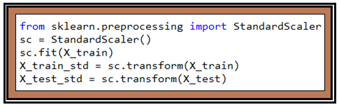
StandardScaler()를 실행한후 sc.fit(X_train) 에 의해 학습용 데타의 평균값 μ와 표준편차 σ를 계산한다. 여기서 사용한 fit() 은 퍼셉트론에서 사용했던 fit()과는 서로 다음에 주의하자. 이들 값을 사용하여 학습용 데이터와 테스트용 데이터를 각각 표준화하도록 하며 여기까지가 데이터의 preprocessing 단계이다.
데이터 준비가 완료되었으면 우선 Perceptron 라이브러리를 불러 적용해 보자. 앞장에서 class Perceptron() 의 세부적인 설명이 이루어졌는데 이 class 는 sklearn 의 lenear_model 중의 하나로서 라이브러리화 되어 있어 편리하게 사용할 수 있다. 학습횟수 n_iter=40, learning rate eth0=0.1 로 두고 미리 준비해 두었던 70%의 X_train_std 와 y_train을 사용하여 학습을 시키자. 학습이 완료되면 내부적으로 계산된 웨이트 값들을 사용해 테스트 데아타를 학습시켜 보아 인식률을 체크해 보기로 한다.
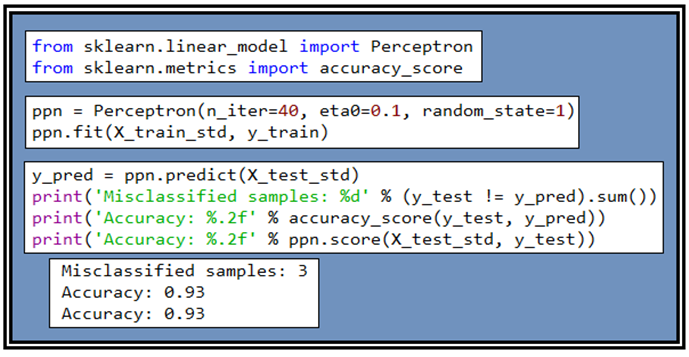
Perceptron을 사용하여 70%에 해당하는 데이터를 학습시켜 웨이트 값들을 얻어내 후 준비해둔 30% 의 테스트 데이터 즉 45개의 샘플을 학습 시킨 결과와 원래 알고 있던 데이터를 비교해보면 3경우(Misclassified)가 즉 6.7%가 틀리게 판명되었으므로 정밀도는 93.3%가 된다.
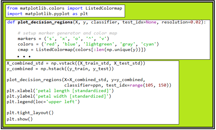
컬러 맵을 작성하는 ListedColormap 부분도 다음과 같이 라이브러리화 되어 있다. 하지만 영역별 색상을 입혀주는 plot_decision_regions 는 라이브러리화 하기 힘든 부분이 있으므로 필요한 파라메터들을 수정한 후 함수로 넣어두고 불러 쓰도록 한다.
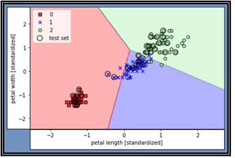
학습결과와 테스트 결과를 함께 작도한 결과이다 색깔별 경계 부분을 월경한 상태의 잘못 분류된 데이터들이 나타나 있다. 이미 지적했지만 퍼셉트론은 “linearly separable” 한 경우에만 100% 정답을 주며 지금의 문제에서처럼 몇 개의 데이터가 지나치게 근접하여 섞여 있는 경우 분리 식별이 곤란해진다. 이 문제를 해결하기 위해 어떤 해결책들이 제시되었는지 Multiclass Logistic regression 편을 통해서 알아보기로 하자.
#ch03_data_read_1_1.py
from sklearn import datasets
import numpy as np
iris = datasets.load_iris()
X = iris.data[:, [2, 3]]
y = iris.target
print('Class labels:', np.unique(y))
from sklearn.model_selection import train_test_split
X_train, X_test, y_train, y_test = train_test_split(
X, y, test_size=0.3, random_state=1, stratify=y)
print('Labels counts in y:', np.bincount(y))
print('Labels counts in y_train:', np.bincount(y_train))
print('Labels counts in y_test:', np.bincount(y_test))
from sklearn.preprocessing import StandardScaler
sc = StandardScaler()
sc.fit(X_train)
X_train_std = sc.transform(X_train)
X_test_std = sc.transform(X_test)
#Training a perceptron via scikit-learn
from sklearn.linear_model import Perceptron
from sklearn.metrics import accuracy_score
ppn = Perceptron(n_iter=40, eta0=0.1, random_state=1)
ppn.fit(X_train_std, y_train)
y_pred = ppn.predict(X_test_std)
print('Misclassified samples: %d' % (y_test != y_pred).sum())
print('Accuracy: %.2f' % accuracy_score(y_test, y_pred))
print('Accuracy: %.2f' % ppn.score(X_test_std, y_test))
from matplotlib.colors import ListedColormap
import matplotlib.pyplot as plt
def plot_decision_regions(X, y, classifier, test_idx=None, resolution=0.02):
#setup marker generator and color map
markers = ('s', 'x', 'o', '^', 'v')
colors = ('red', 'blue', 'lightgreen', 'gray', 'cyan')
cmap = ListedColormap(colors[:len(np.unique(y))])

#plot the decision surface
x1_min, x1_max = X[:, 0].min() - 1, X[:, 0].max() + 1
x2_min, x2_max = X[:, 1].min() - 1, X[:, 1].max() + 1
xx1, xx2 = np.meshgrid(np.arange(x1_min, x1_max, resolution),
                       np.arange(x2_min, x2_max, resolution))
Z = classifier.predict(np.array([xx1.ravel(), xx2.ravel()]).T)
Z = Z.reshape(xx1.shape)
plt.contourf(xx1, xx2, Z, alpha=0.3, cmap=cmap)
plt.xlim(xx1.min(), xx1.max())
plt.ylim(xx2.min(), xx2.max())

for idx, cl in enumerate(np.unique(y)):
    plt.scatter(x=X[y == cl, 0],
                y=X[y == cl, 1],
                alpha=0.8,
                c=colors[idx],
                marker=markers[idx],
                label=cl,
                edgecolor='black')

#highlight test samples
if test_idx:
    #plot all samples
    X_test, y_test = X[test_idx, :], y[test_idx]

    plt.scatter(X_test[:, 0],
                X_test[:, 1],
                c='',
                edgecolor='black',
                alpha=1.0,
                linewidth=1,
                marker='o',
                s=100,
                label='test set')
#Training a perceptron model using the standardized training data:
X_combined_std = np.vstack((X_train_std, X_test_std))
y_combined = np.hstack((y_train, y_test))
plot_decision_regions(X=X_combined_std, y=y_combined,
classifier=ppn, test_idx=range(105, 150))
plt.xlabel('petal length [standardized]')
plt.ylabel('petal width [standardized]')
plt.legend(loc='upper left')
plt.tight_layout()
plt.show()
짱짱맨 호출에 응답하여 보팅하였습니다.