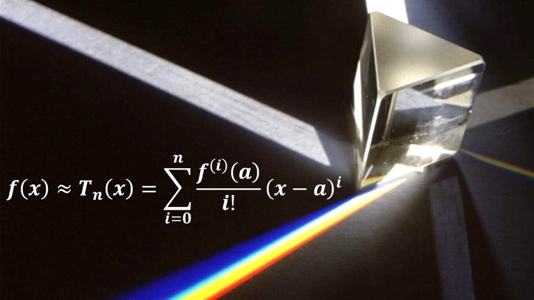
In this video I go over further into infinite sequences and series, and this time look at the many applications of Taylor polynomials. When I was still a student in university, it was this particular concept of Taylor polynomials and their applications to all aspects of physics that got me interested in creating my Math Easy Solutions channel. And in this video I explore Taylor polynomials in approximating functions which can then be extended to most functions in physics.
The accuracy of our approximations can be determined using the Alternating Series Estimation theorem, Taylor's Inequality, and through graphical or even brute force calculation methods. The particular science and physics applications that I cover in this video include optics, electromagnetism, water waves, pendulums, and surveying.
The topics covered in this video are listed below with their time stamps.
- @ 1:04 - Topics to Cover
- @ 2:18 - Introduction
- @ 2:48 - Recap on Power Series and Taylor Polynomials
- @ 8:22 - Approximating Functions by Polynomials
- @ 30:37 - Example 1: f(x) = x1/3
- Example 2: f(x) = sin x
- @ 53:48 - Using Alternating Series Estimation Theorem
- @ 1:14:22 - Using Taylor's Inequality
- @ 1:21:11 - Using Graphical Methods
- @ 1:32:04 - Applications to Physics
- @ 1:32:38 - Example 3: Einstein's Theory of Special Relativity
- @ 2:02:16 - Optical Physics
- @ 2:21:25 - Exercises
- @ 2:21:42 - Exercise 1: Taylor Derivatives
- @ 2:30:50 - Exercise 2: Optical Physics
- @ 3:19:35 - Exercise 3: Electric Dipoles
- @ 3:33:36 - Exercise 4: Water Waves
- @ 4:09:52 - Exercise 5: Pendulum Period
- @ 4:52:04 - Exercise 6: Surveying
Watch Video On:
- 3Speak: https://3speak.tv/watch?v=mes/gucinser
- Odysee: https://odysee.com/@mes:8/1033-Appliations-of-Taylor-Polynomials:9
- BitChute: https://www.bitchute.com/video/szxFhvDiahLL/
- Rumble: https://rumble.com/v1q7a12-infinite-sequences-and-series-applications-of-taylor-polynomials.html
- DTube: https://d.tube/#!/v/mes/jqqdqrhbdaq
- YouTube: https://youtu.be/Tuh3Ht4XwYI
Download Video Notes: https://1drv.ms/b/s!As32ynv0LoaIiMQFpSc5JN-fpBUyHw?e=sQWbWc
View Video Notes Below!
Download these notes: Link is in video description.
View these notes as an article: https://peakd.com/@mes
Subscribe via email: http://mes.fm/subscribe
Donate! :) https://mes.fm/donate
Buy MES merchandise! https://mes.fm/storeReuse of my videos:
- Feel free to make use of / re-upload / monetize my videos as long as you provide a link to the original video.
Fight back against censorship:
- Bookmark sites/channels/accounts and check periodically
- Remember to always archive website pages in case they get deleted/changed.
Buy "Where Did The Towers Go?" by Dr. Judy Wood: https://mes.fm/judywoodbook
Subscribe to MES Truth: https://mes.fm/truthJoin my forums!
- Hive community: https://peakd.com/c/hive-128780
- Reddit: https://reddit.com/r/AMAZINGMathStuff
- Voat: https://voat.co/v/AMAZINGMathStuff
- Discord: https://mes.fm/chatroom
Follow along my epic video series:
- #MESScience: https://mes.fm/science-playlist
- #MESExperiments: https://peakd.com/mesexperiments/@mes/list
- #AntiGravity: https://peakd.com/antigravity/@mes/series
-- See Part 6 for my Self Appointed PhD and #MESDuality breakthrough concept!- #FreeEnergy: https://mes.fm/freeenergy-playlist
- #PG (YouTube-deleted series): https://peakd.com/pg/@mes/videos
NOTE #1: If you don't have time to watch this whole video:
- Skip to the end for Summary and Conclusions (if available)
- Play this video at a faster speed.
-- TOP SECRET LIFE HACK: Your brain gets used to faster speed!
-- Browser extension recommendation: https://mes.fm/videospeed-extension
-- See my tutorial to learn more: https://peakd.com/video/@mes/play-videos-at-faster-or-slower-speeds-on-any-website- Download and read video notes.
- Read notes on the Hive blockchain #Hive
- Watch the video in parts.
-- Timestamps of all parts are in the description.Browser extension recommendations:
- Increase video audio: https://mes.fm/volume-extension
- Text to speech: https://mes.fm/speech-extension
Infinite Sequences and Series: Applications of Taylor Polynomials
Calculus Book Reference
Note that I mainly follow along the following calculus book:
Calculus: Early Transcendentals Sixth Edition by James Stewart
Topics to Cover
- Introduction
- Recap on Power Series and Taylor Polynomials
- Approximating Functions by Polynomials
- Example 1: f(x) = x1/3
- Example 2: f(x) = sin x
- Using Alternating Series Estimation Theorem
- Using Taylor's Inequality
- Using Graphical Methods
- Applications to Physics
- Example 3: Einstein's Theory of Special Relativity
- Optical Physics
- Exercises
- Exercise 1: Taylor Derivatives
- Exercise 2: Optical Physics
- Exercise 3: Electric Dipoles
- Exercise 4: Water Waves
- Exercise 5: Pendulum Period
- Exercise 6: Surveying
Introduction
In this section we explore two types of applications of Taylor polynomials.
First we look at how they are used to approximate functions -- computer scientists like them because polynomials are the simplest of functions.
Then we investigate how physicists and engineers use them in such fields as relativity, optics, blackbody radiation, electric dipoles, the velocity of water waves, and building highways across a desert.
Recap on Power Series and Taylor Polynomials
Here is a recap of power series, which are a specific type of series.
https://peakd.com/mathematics/@mes/infinite-sequences-and-series-power-series
Retrieved: 6 August 2020
Archive: https://archive.vn/mpruy
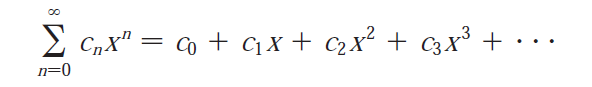
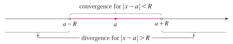
Power series centered at a:
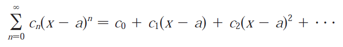
The convention (x - a)0 = 1 is used even when x = a.
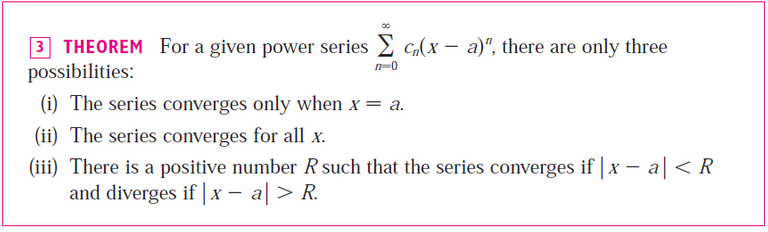
Note that R is the radius of convergence; R = a for (i) and R = ∞ for (ii).
When |x - a| = R, i.e. at the endpoints of the interval of convergence x = a ± R, then the series may converge or may diverge.
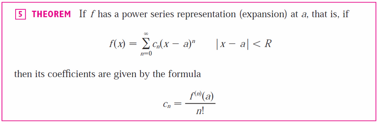
Recall that the Taylor series is just a power series in which the coefficients are determined from the function's derivatives.
https://peakd.com/mathematics/@mes/infinite-sequences-and-series-taylor-and-maclaurin-series
Retrieved: 24 September 2020
Archive: https://archive.is/w3n31
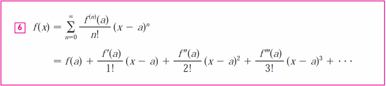
The Maclaurin series is a just a specific type of Taylor series with a = 0:

A function is equal to its Taylor series when the remainder approaches 0:
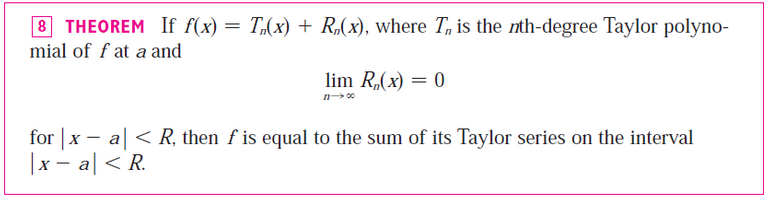
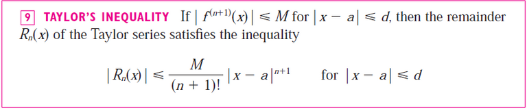
Taylor's Inequality is used to evaluate the remainder:
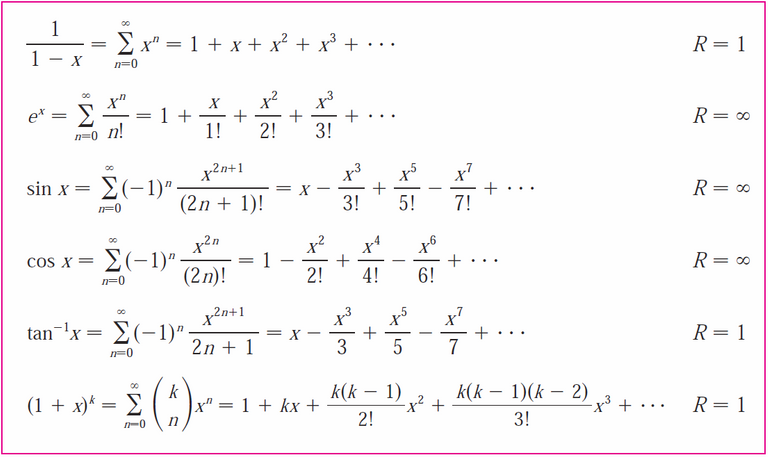
Here are several common functions and their Maclaurin series:
Table 1:
Approximating Functions by Polynomials
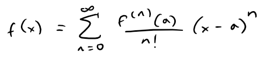
Suppose that f(x) is equal to the sum of its Taylor series at a:
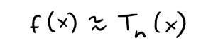
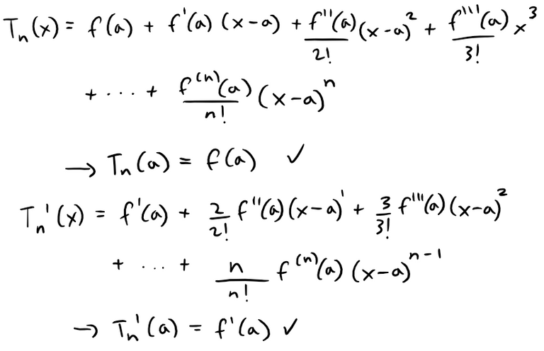
In my earlier video, referenced in the Recap section above, we introduced the notation Tn(x) for the n-th partial sum of this series and called it the n-th degree Taylor polynomial of f at a.
Thus:
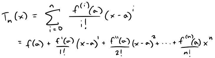
Since f is the sum of its Taylor series, we know that Tn(x) → f(x) as n → ∞ and so Tn can be used as an approximation to f:
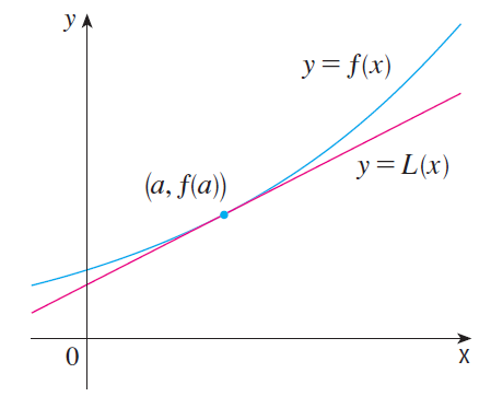
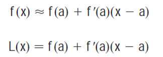
Notice that the first-degree Taylor polynomial:
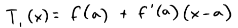
is the same as the linearization or linear approximation of f at a that we discussed in my earlier video, referenced below.
Retrieved: 28 November 2020
Video notes archive: https://archive.vn/QYUsw
Notice also that T1 and its derivative have the same values at a that f and f' have.
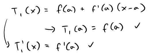
In general, it can be shown that the derivatives of Tn at a agree with those of f up to and including derivatives of order n, see Exercise 1 at the end of this video.
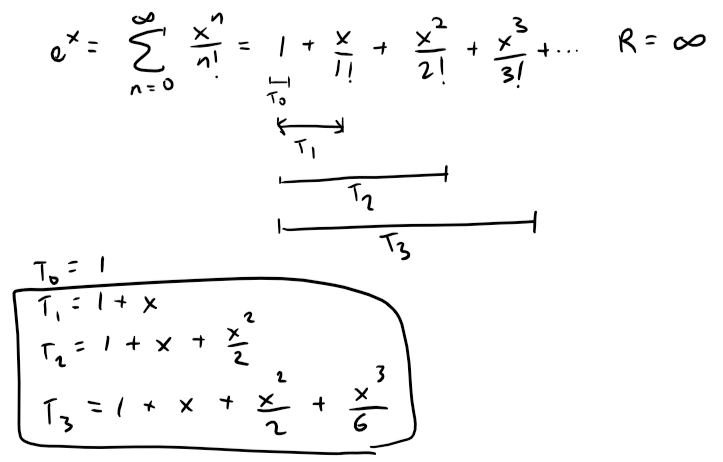
To illustrate these ideas let's take a look at the graphs of y = ex and its first few Taylor polynomials centered at x = a = 0, thus y = e0 = 1 and the point becomes (0, 1).
First, recall the Maclaurin series for ex and the corresponding first three partial sums:
Using the same Desmos graph from my earlier video on Taylor polynomials, we can see that the higher degree Taylor or Maclaurin polynomials are more in line with the ex.
https://www.desmos.com/calculator/vqtlbufbnn
Retrieved: 17 January 2020
Archive: https://archive.ph/wip/EA87o
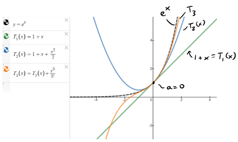
The graph of T1 is the tangent line to y = ex at (0, 1); this tangent line is the best linear approximation to ex near (0, 1).
The graph of T2 is the parabola y = 1 + x + x2/2, and the graph of T3 is the cubic curve y = 1 + x + x2/2 + x3/6, which is a closer fit to the exponential curve y = ex than T2.
The next Taylor polynomial T4 would be an even better approximation, and so on.
The values in the table below give a numerical demonstration of the convergence of the Taylor polynomials Tn(x) to the function y = ex.
https://1drv.ms/x/s!As32ynv0LoaIiMQd31Z5qwO1xuXqpA?e=zGdg1x
Retrieved: 28 November 2020
Archive: Not available
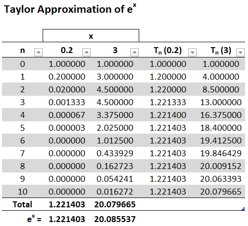
We see that when x = 0.2 the convergence is very rapid, but when x = 3 it is somewhat slower.
In fact, the farther x is from 0, the more slowly Tn(x) converges to ex.
When using a Taylor polynomial Tn to approximate a function f, we have to ask the questions:
How good an approximation is it?
How large should we take n to be in order to achieve a desired accuracy?
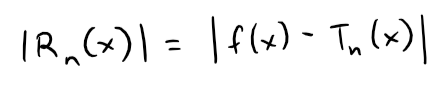
To answer these question we need to look at the absolute value of the remainder:
There are three possible methods for estimating the size of the error:
- If a graphing device is available, we can use it to graph |Rn(x)| and thereby estimate the error.
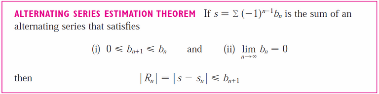
- If the series happens to be an alternating series, we can use the Alternating Series Estimation Theorem.
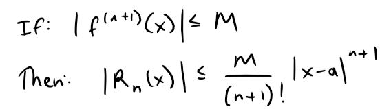
- In all cases we can use Taylor's Inequality, which says that:
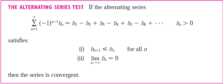
Recall the Alternating Series Test and Estimation Theorem from my earlier video.
https://peakd.com/mathematics/@mes/infinite-sequences-and-series-alternating-tests
Retrieved: 29 November 2020
Archive: https://archive.vn/wip/iFUns
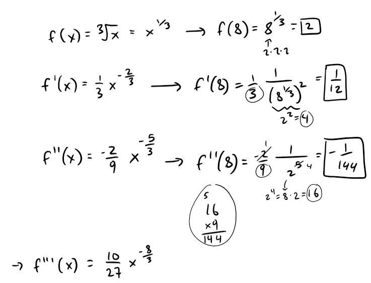
Example 1
(a) Approximate the following function by a Taylor polynomial of degree 2 at a = 8.
(b) How accurate is this approximation when 7 ≤ x ≤ 9?
Solution:
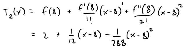
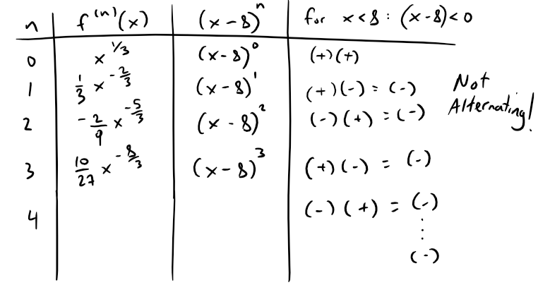
(a) Let's obtain the first 3 derivatives of f at a:
Thus the second-degree Taylor polynomial is:
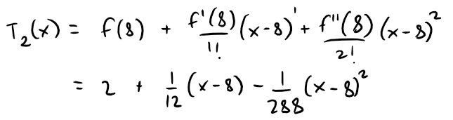
The desired approximation is:
(b) Note that the Taylor series is not alternating when x < 8, so we can't use the Alternating Series Estimation Theorem in this example.
But we can use Taylor's Inequality with n = 2 and a = 8:
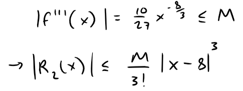
Because x ≥ 7, we have x8/3 ≥ 78/3 and so:
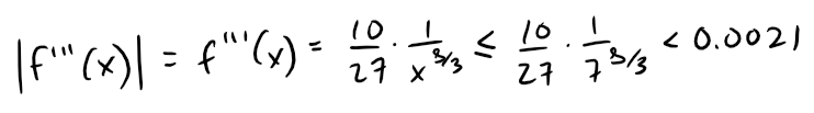
Calculation Check: 10/27 * 1/7^(8/3) = 0.0021
Therefore we can take M = 0.0021.
Also, our given interval obtains:
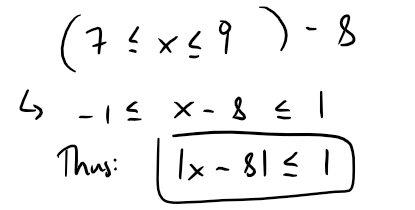
Then Taylor's Inequality gives:
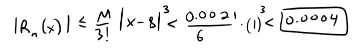
Calculation Check: 0.0021/6 = 0.0004
Thus, if 7 ≤ x ≤ 9, the approximation in part (a) is accurate to within 0.0004.
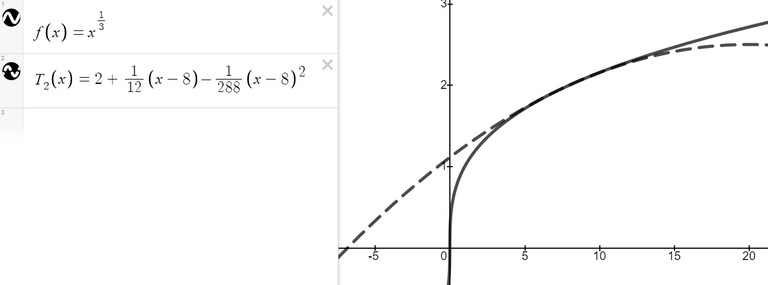
Let's use graphing device to check the calculation in Example 1.
The figure below shows that the graphs of f(x) and T2(x) are very close to each other when x is near 8.
https://www.desmos.com/calculator/grpvrbzkqp
Retrieved: 30 November 2020
Archive: https://archive.vn/wip/wNgvO
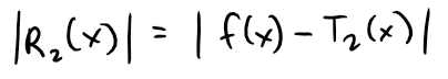
We can also graph the remainder computed from the expression:
https://www.desmos.com/calculator/wvdwj2uval
Retrieved: 30 November 2020
Archive: https://archive.vn/IvJLB
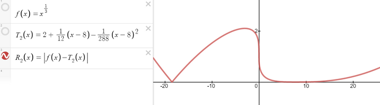
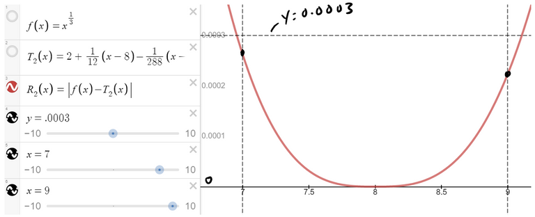
We see from the graph that:
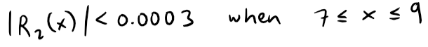
Thus the error estimate from graphical methods is slightly better than the error estimate from Taylor's Inequality in this case.
Example 2
(a) What is the maximum error possible in using the approximation below?
Use this approximation to find sin 12° correct to six decimal places.
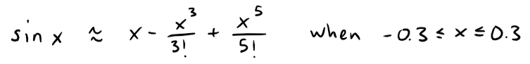
(b) For what values of x is this approximation accurate to within 0.00005?
Solution:
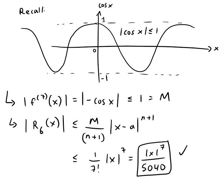
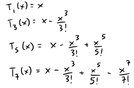
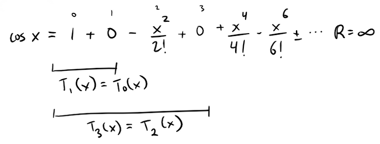
Recall the Maclaurin series for sin x listed in the earlier Table 1:
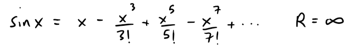
Note that this series is alternating for all nonzero values of x:
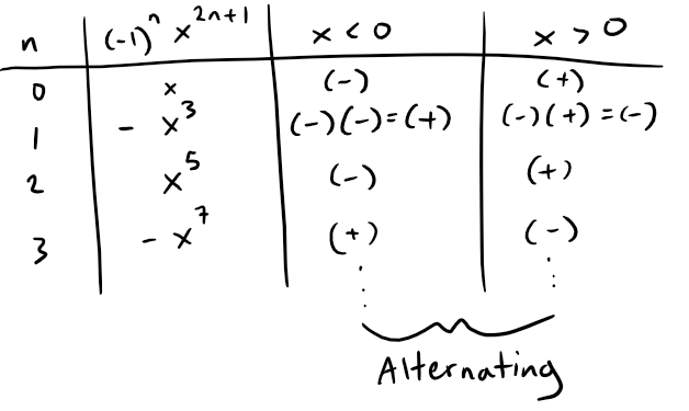
The successive terms decrease in size because |x| < 1 and their limit approaches 0, so we can use the Alternating Series Estimation Theorem.
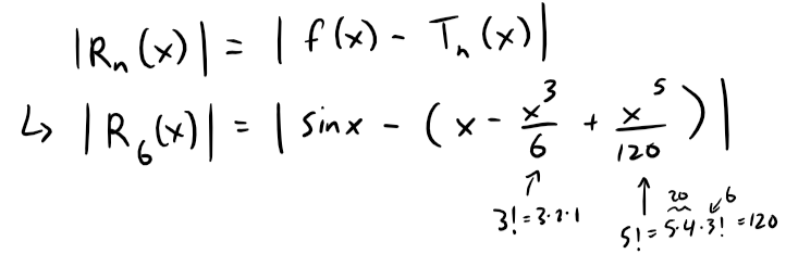
The error in approximating sin x by the first three terms of its Maclaurin series is at most:
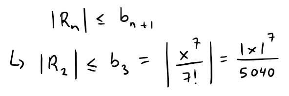
Calculation Check: 7! = 5,040
If -0.3 ≤ x ≤ 0.3, then |x| ≤ 0.3, so the error is smaller than:
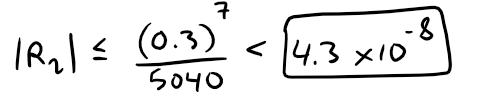
Calculation Check:
https://duckduckgo.com/?q=0.3%5E7%2F5040&t=h_&ia=calculator
Retrieved: 30 November 2020
Archive: https://archive.vn/wip/YU0NA
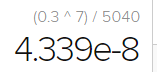
MES Note: Most calculators use the notation, for example, e-8 as being 10-8.
To find sin 12° we first convert to radians.
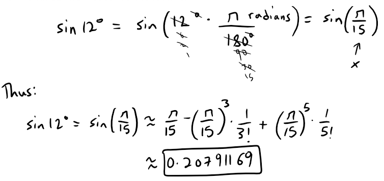
Calculation Check:
- Pi/15 - (pi/15)^3 * 1/3! + (pi/15)^5 * 1/5! = 0.207911694322979
- Sin(12) = 0.207911690817759
Thus, correct to six decimal places, since our estimated error is within 8 decimal places, we have sin 12° ≈ 0.207912.
(b) The error will be smaller than 0.00005 if:
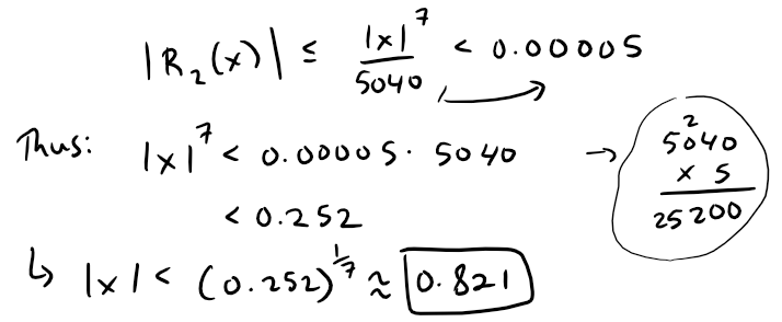
Calculation Check:
- 0.252^(1/7) = 0.8213
- 0.00005 * 5040 = 0.252
So the given approximation is accurate to within 0.00005 when |x| < 0.82.
What If We Use Taylor's Inequality to Solve Example 2?
Solving for the derivatives of sin x we get:
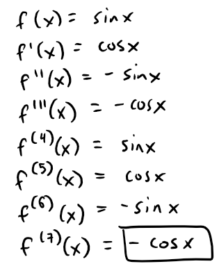
Since cosine and sine functions oscillate between -1 and 1, we can apply Taylor's Inequality accordingly:
This is the same as before, thus we get the same estimates as with the Alternating Series Estimation Theorem.
What About Graphical Methods?
We can graph the following Remainder function:
We can graph the Remainder and compare it to the maximum error determined in Example 2 (a).
https://www.desmos.com/calculator/yphi6wpizp
Retrieved: 30 November 2020
Archive: https://archive.vn/uBfTI
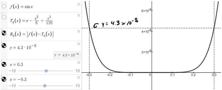
We can see from it that |R6(x)| < 4.3 x 10⁻⁸ when |x| ≤ 0.3.
This is the same estimate that we obtained in Example 2 (a).
For part (b) we want |R6(x)| < 0.00005, so we graph both y = |R6(x)| and y = 0.00005 in the figure below.
https://www.desmos.com/calculator/5uuyhdlp1y
Retrieved: 20 November 2020
Archive: https://archive.vn/wip/HfFPF
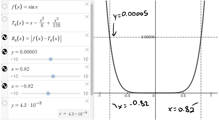
Plotting x = ± 0.82 we can find that the inequality is satisfied when |x| < 0.82.
Again this is the same estimate that we obtained in the solution to Example 2 (b).
If we had been asked to approximate sin 72° instead of sin 12° in Example 2, it would have been wise to use the Taylor polynomials at a = π/3 (instead of a = 0) because they are better approximations to sin x for values of x close to π/3.
Notice that 72° is close to 60° (or π/3 radians) and the derivatives of sin x are easy to compute at π/3.
We can graph the following Maclaurin polynomial approximations for sin x:
https://www.desmos.com/calculator/8pl3nc2zha
Retrieved: 8 December 2020
Archive: https://archive.vn/lwL83
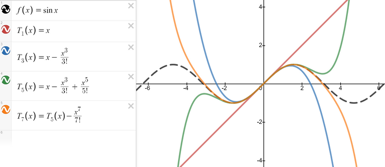
You can see that as n increases, Tn(x) is a good approximation to sin x on a larger and larger interval.
One use of the type of calculation done in Examples 1 and 2 occurs in calculators and computers.
For instance, when you press the sin or ex keys on your calculator, or when a computer programmer uses a subroutine for a trigonometric or exponential or Bessel function, in many machines a polynomial approximation is calculated.
The polynomial is often a Taylor polynomial that has been modified so that the error is spread more evenly throughout an interval.
Applications to Physics
Taylor polynomials are also used frequently in physics.
In order to gain insight into an equation, a physicist often simplifies a function by considering only the first two or three terms in its Taylor series.
In other words, the physicist uses a Taylor polynomial as an approximation to the function.
Taylor's Inequality can then be used to gauge the accuracy of the approximation.
The following example shows one way in which this idea is used in special relativity.
Example 3
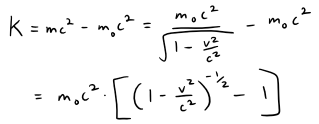
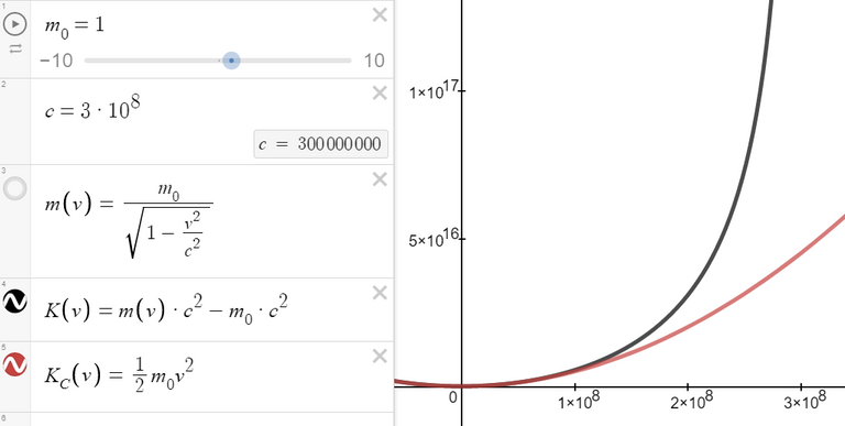
In Einstein's theory of special relativity the mass of an object moving with velocity v is:
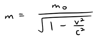
Where m0 is the mass of the object when at rest and c is the speed of light.
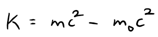
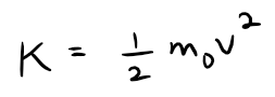
The kinetic energy of the object is the difference between its total energy and its energy at rest:
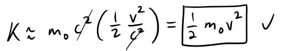
(a) Show that when v is very small compared with c, this expression for K agrees with classical Newtonian physics:
(b) Use Taylor's Inequality to estimate the difference in these expressions for K when |v| ≤ 100 m/s.
Solution:
(a) Using the expressions given for K and m, we get:
With x = -v2/c2, the Maclaurin series for (1 + x)-1/2 is most easily computed as a binomial series with k = -1/2.
Notice that |x| < 1 because v < c.
Therefore we have:
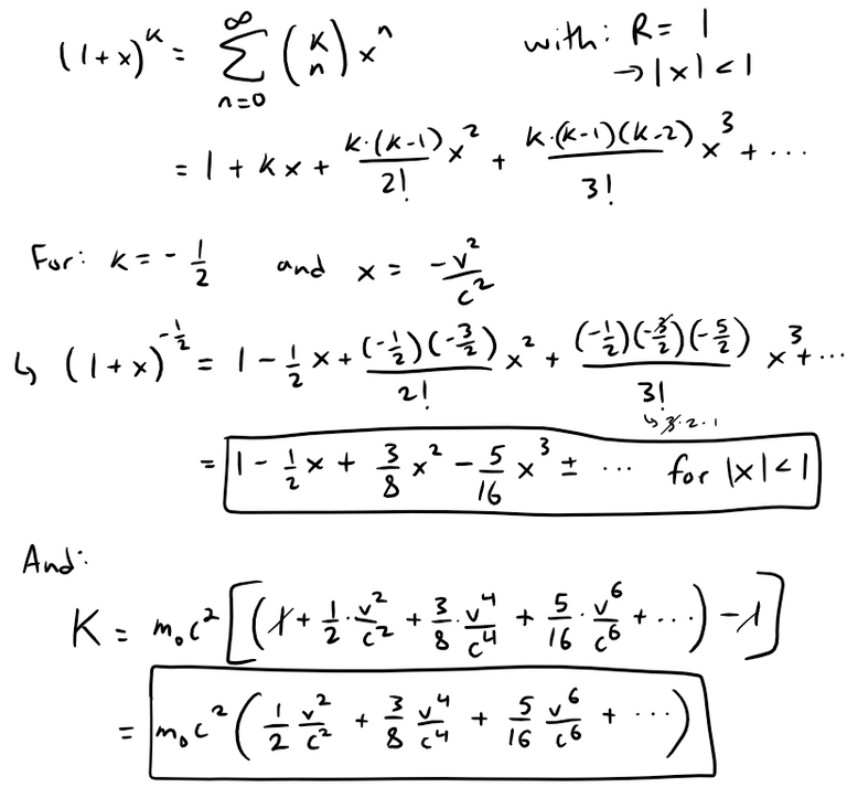
If v is much smaller than c, then all terms after the first are very small when compared with the first term.
If we omit them, we get:
(b) We can use Taylor's Inequality to estimate the Remainder R1(x) as follows, since our above derivation for K involved just the first two terms of the Maclaurin series (that is n = 1):
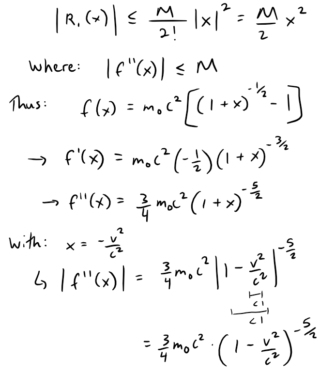
Since we are given that |v| ≤ 100 m/s, so we have:
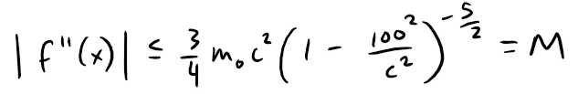
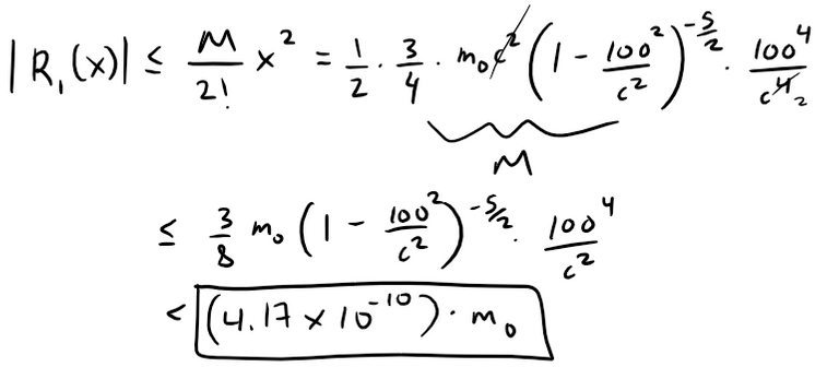
Thus, with c = 3 x 10⁸ m/s, we get:
Calculation Check:
https://tinyurl.com/calculationcheck1
Retrieved: 1 December 2020
Archive: https://archive.vn/iaq3L
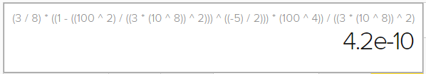
So when |v| ≤ 100 m/s, the magnitude of the error in using the Newtonian expression for kinetic energy is at most (4.2 x 10⁻¹⁰) · m0.
The upper curve in the figure below is the graph of the expression for the kinetic energy K of an object with velocity v in special relativity.
The lower curve shows the function used for K in classical Newtonian physics.
When v is much smaller than the speed of light, the curves are practically identical.
https://www.desmos.com/calculator/qhskha70eg
Retrieved: 9 December 2020
Archive: https://archive.vn/wip/INXCS
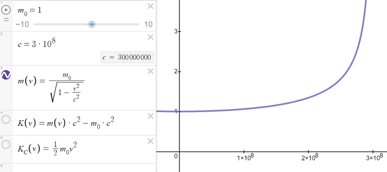
Note also how the mass formula of a moving object rises to infinity as the speed approaches the speed of light.
https://www.desmos.com/calculator/0limsnshiy
Retrieved: 9 December 2020
Archive: https://archive.vn/wip/36oIJ
Optical Physics
Another application to physics occurs in optics.
The figure below depicts a wave from the point source S meeting a spherical interface of radius R centered at C.
The ray SA is refracted (or passes through the spherical interface) toward P.
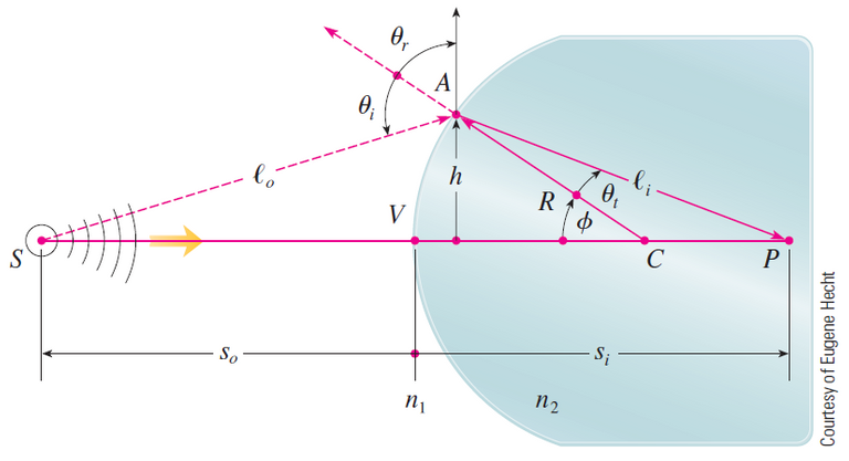
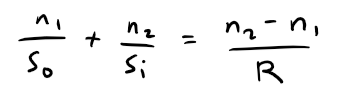
Using Fermat's principle that light travels so as to minimize the time taken, the author of the image Eugene Hecht derives the equation:
Equation 1:
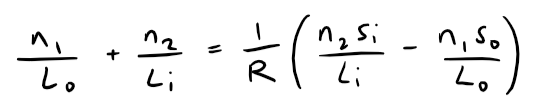
Where n1 and n2 are indices of refraction and L0, Li, s0, and si are the distances indicated in the figure.
Note that the index of refraction is the ratio of the speed of light in a vacuum over the speed of light in the medium, that is n = c/v.
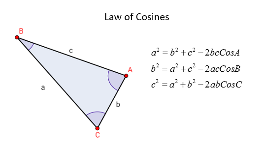
By the Law of Cosines, referenced from my earlier video below, we can determine the lengths L0 and Li from the triangles ACS and ACP.
https://youtu.be/wOCYb3Ku6yw
Retrieved: 1 December 2020
Video notes archive: https://archive.vn/wip/QfLTc
Thus we can derive the following Equation 2:
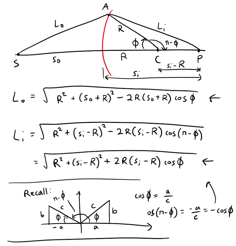
The above Equation 2 makes the earlier Equation 1 cumbersome to work with, which is why Carl Friedrich Gauss, in 1841, simplified it by using the linear approximation cos φ ≈ 1 for small values of φ.
Note that this amounts to using the Taylor polynomial of degree 1 since the odd powers equal to 0.
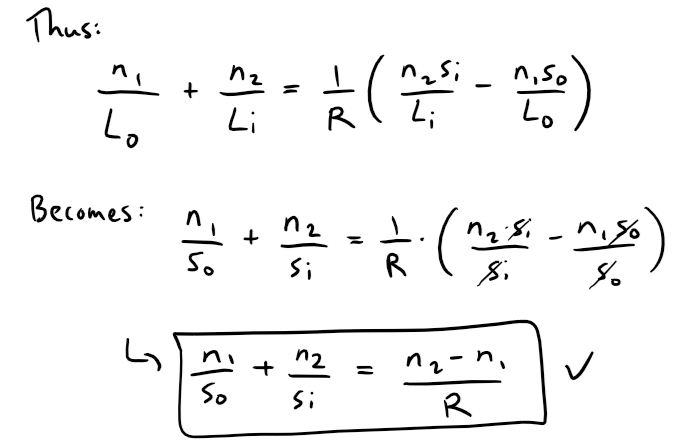
With this approximation Equation 1 becomes the following simpler equation, which we are asked to show in Exercise 2 (a) later in this video.
Equation 3:
The resulting optical theory is known as Gaussian optics, or first-order optics, and has become the basic theoretical tool used to design lenses.
A more accurate theory is obtained by approximating cos φ by its Taylor polynomial of degree 3 (which is the same as the Taylor polynomial of degree 2).
This takes into account rays for which φ is not so small, that is, rays that strike the surface at greater distances h above the axis.
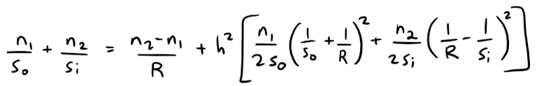
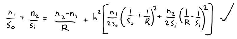
In Exercise 2 (b) we are asked to use this approximation to derive the more accurate equation:
Equation 4:
The resulting optical theory is known as third-order optics.
Other applications of Taylor polynomials to physics and engineering are explored in Exercises that follow and in an Applied Project in a later video.
Exercises
Exercise 1: Taylor Derivatives
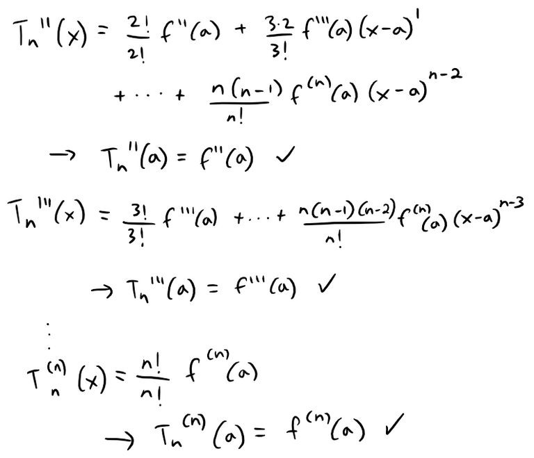
Show that Tn and f have the same derivatives at a up to order n.
Solution:
We can see that the Taylor polynomial and all of its derivatives cancel out all the terms, except the first term, at x = a thus equating to f and its derivatives.
Exercise 2: Optical Physics
(a) Derive Equation 3 for Gaussian optics from Equation 1 by approximating cos φ in Equation 2 by its first-degree Taylor polynomial.
(b) Show that if cos φ is replaced by its third-degree Taylor polynomial in Equation 2, then Equation 1 becomes Equation 4 for third-order optics.
Hint:
Use the first two terms in the binomial series for L-10 and L-1i.
Also, use φ ≈ sin φ.
Solution:
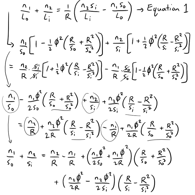
(a) Inserting Equation 2 with cos φ ≈ 1, that is approximating it with its first order Taylor polynomial, into Equation 1 we get:
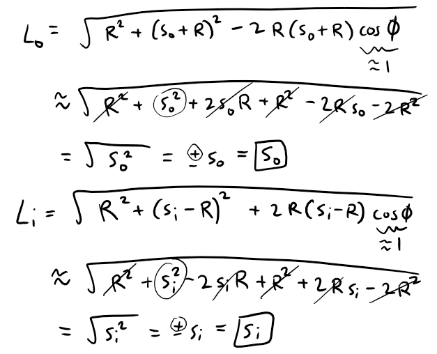
(b) Now let's use the third degree Taylor polynomial for cos φ.
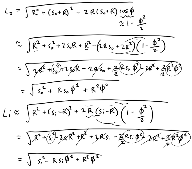
Anticipating that we will use the binomial series expansion from the hint given, we can write our expressions for L0 and Li as follows:
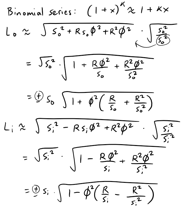
We can now approximate L-10 and L-1i by the first two terms in their binomial series.
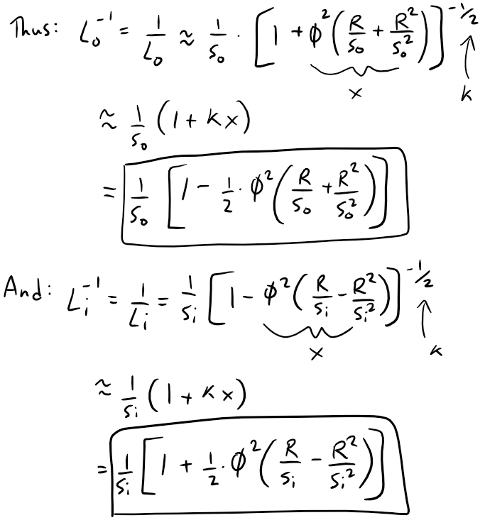
Thus, Equation 1 becomes:
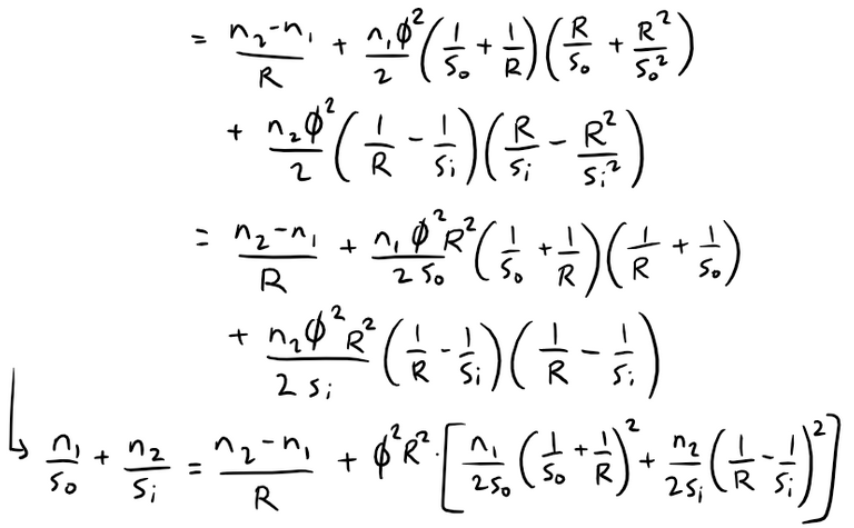
To apply the second hint that we were given, that is to use the approximation φ ≈ sin φ, we first need to look at the refraction figure again.
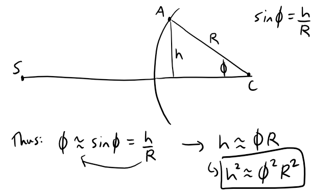
Plugging this into our derived formula above gives us the desired Equation 4.
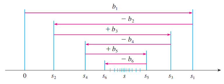
Exercise 3: Electric Dipoles
An electric dipole consists of two electric charges of equal magnitude and opposite sign.
If the charges are q and -q and are located at a distance d from each other, then the electric field E at the point P in the figure is:
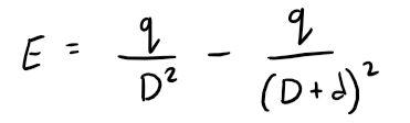
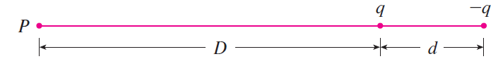
By expanding this expression for E as a series in powers of d/D, show that E is approximately proportional to 1/D3 when P is far away from the dipole.
Solution:
We can rewrite the electric field equation to be able to use the binomial series:
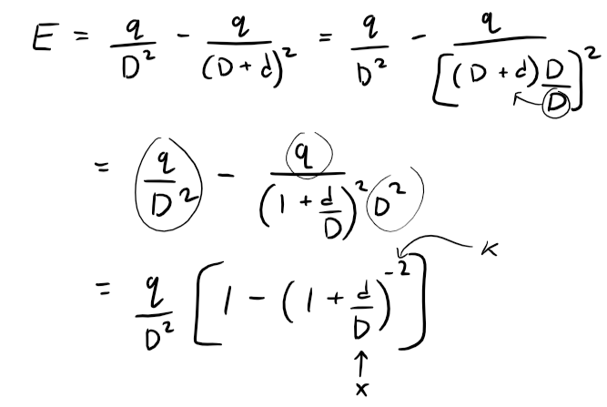
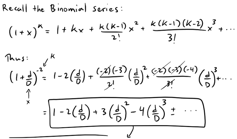
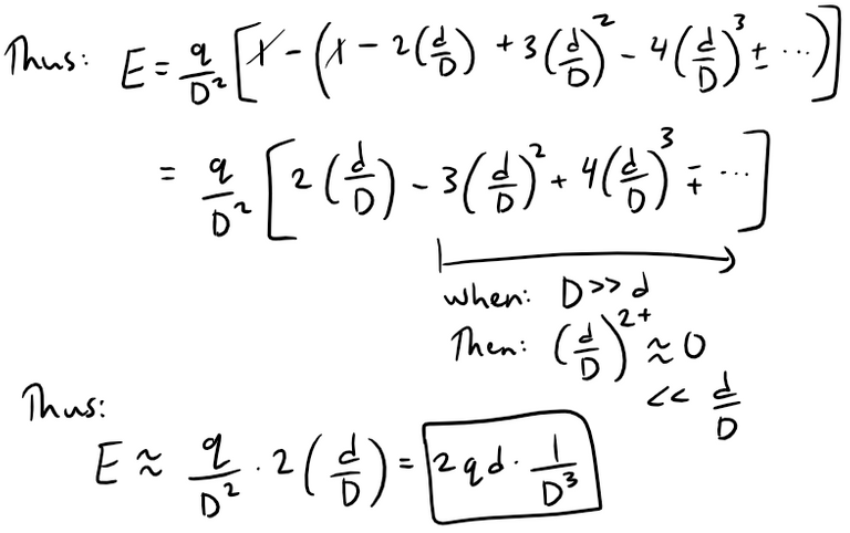
Thus when D >> d, that is when P is far away from the dipole, then E is proportional to 1/D3.
Exercise 4: Water Waves
If a water wave with length L moves with velocity v across a body of water with depth d, as in the figure below, then:
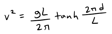
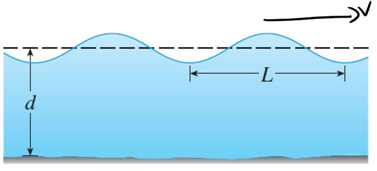
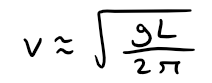
(a) If the water is deep, show that:
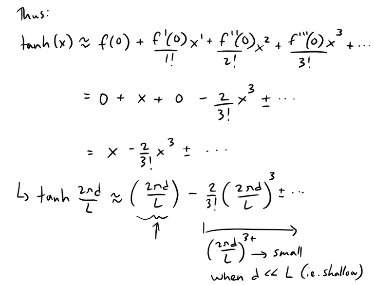
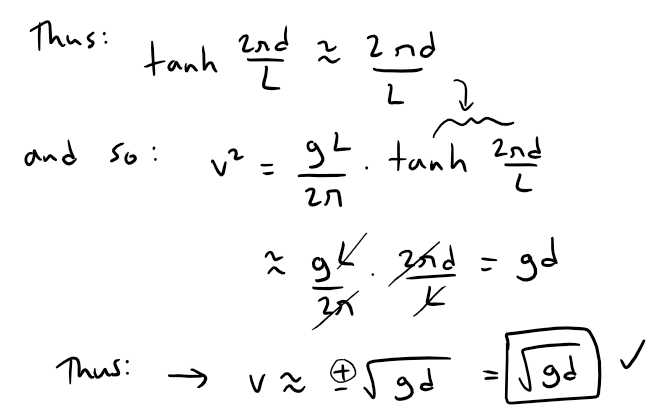
(b) If the water is shallow, use the Maclaurin series for tanh to show that:
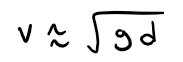
Thus in shallow water the velocity of a wave tends to be independent of the length of the wave.
(c) Use the Alternating Estimation Theorem to show that if L > 10 d, then the estimate v2 ≈ g d is accurate to within 0.014 g L.
Solution:
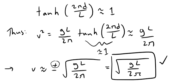
(a) If the water is deep, then 2πd/L is large, and we know from my earlier video referenced below that tanh x → 1 as x → ∞.
https://youtu.be/EmJKuQBEdlc
Retrieved: 23 September 2020
Notes archive: https://archive.vn/wip/6Yin5
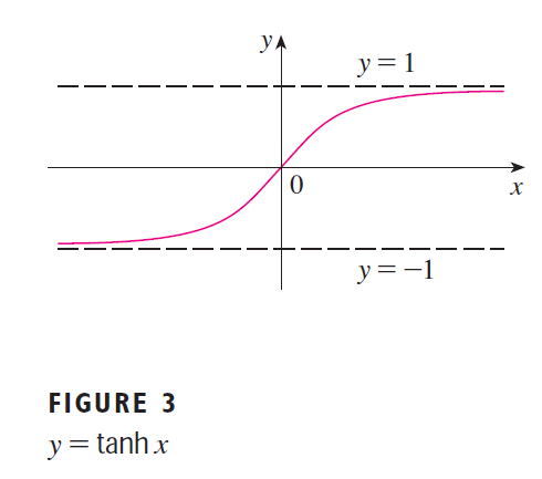
Thus we can use the following approximation for when the water is deep.
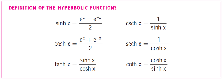
(b) The Maclaurin series requires the derivatives at x = 0, which we can determine for tanh by first recalling the derivatives (and identities) of hyperbolic functions from my earlier video.
https://www.youtube.com/playlist?list=PL328F7D902A09B019
Retrieved: 4 December 2020
Archive: https://archive.vn/wip/lIC7V
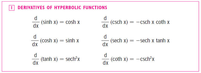
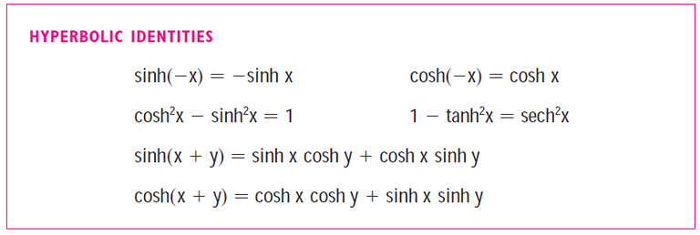
Thus we have:
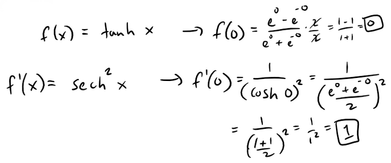
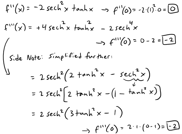
Thus, from the derivatives the first term in the Maclaurin series of tanh x is x, so if the water is shallow, we can use the following approximation:
(c) MES Note: Although the exercise implies that the Maclaurin series for tanh x is alternating I couldn't obtain a formal proof and I am not sure what my calculus book Solutions Manual means by their sentence:
"Since tanh x is an odd function, its Maclaurin series is alternating…"
I will look into this in the future!
Recall the Alternating Series Estimation Theorem:
https://peakd.com/mathematics/@mes/infinite-sequences-and-series-alternating-tests

Thus our estimation for tanh x has a remainder less than the first neglected term of the series.
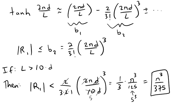
We can now estimate the accuracy of our approximation v2 ≈ g d:
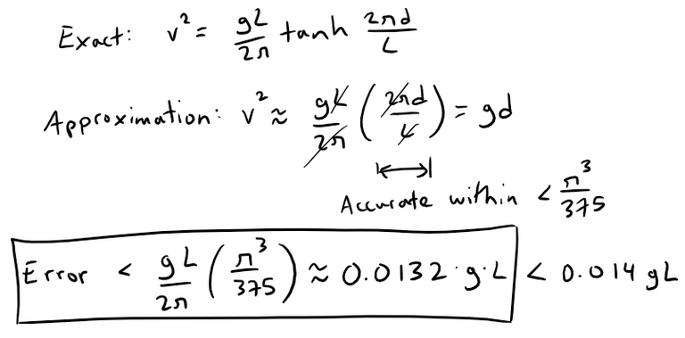
Calculation Check: pi^3 / (2 * pi * 375) = 0.0131594725347858
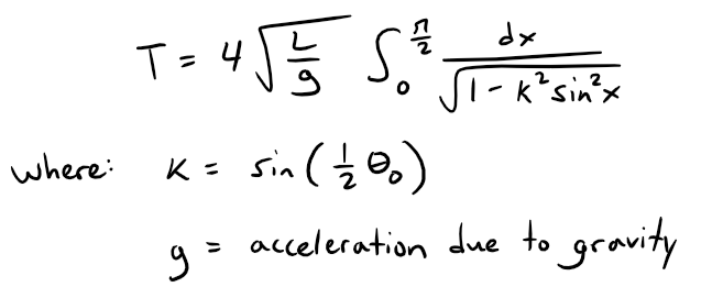
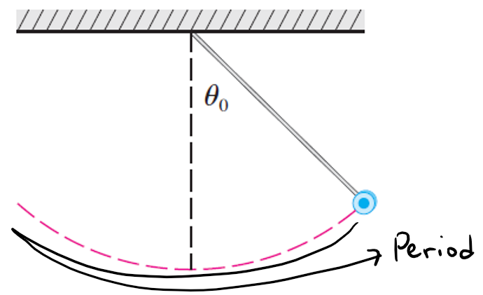
Exercise 5: Pendulum Period
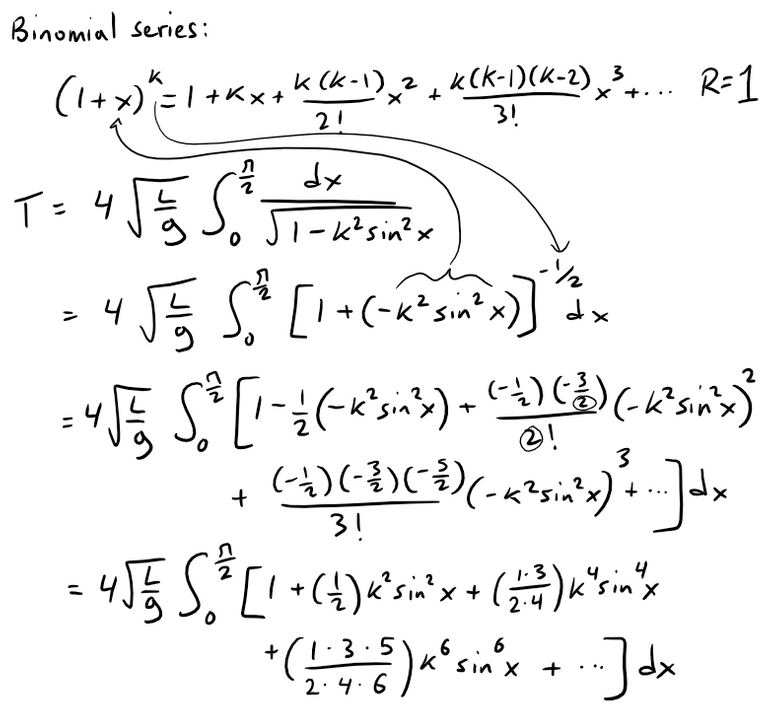
The period of a pendulum with length L that makes a maximum angle θ0 with the vertical is:
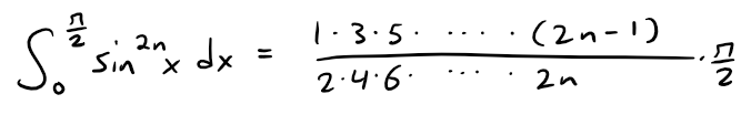
(a) Expand the integrand as a binomial series to show that:
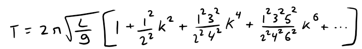
Use the following formula in the derivation (which I may or may not prove in a later video):
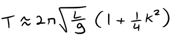
If θ0 is not too large, the approximation T ≈ 2π (L/g)1/2, obtained by using only the first term in the series, is often used.
A better approximation is obtained by using two terms:
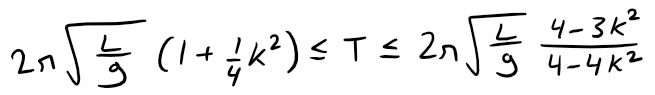
(b) Notice that all terms in the series after the first one have coefficients that are at most 1/4.
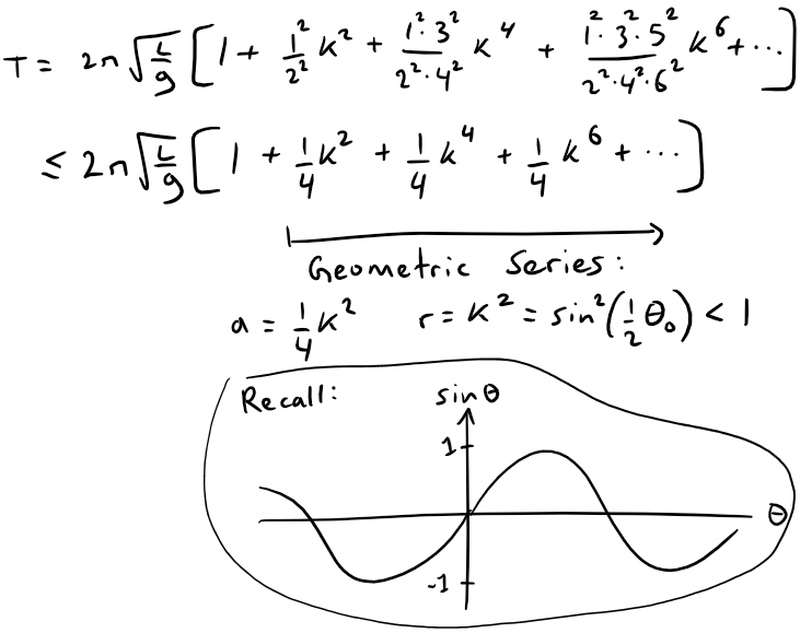
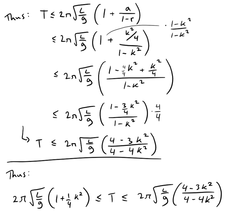
Use this fact to compare this series with a geometric series and show that:
(c) Use the inequalities in part (b) to estimate the period of a pendulum with L = 1 meter and θ0 = 10°.
How does it compare with the estimate T ≈ 2π (L/g)1/2?
What if θ0 = 42°?
Solution:
(a) Let's first write this out in the usual binomial series form:
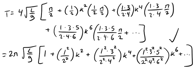
Now we can use our given formula for the integral of sin2n(x) and evaluate the integral term by term from 0 to π/2:
(b) The first of the two inequalities is true because all of the terms in the series are positive.
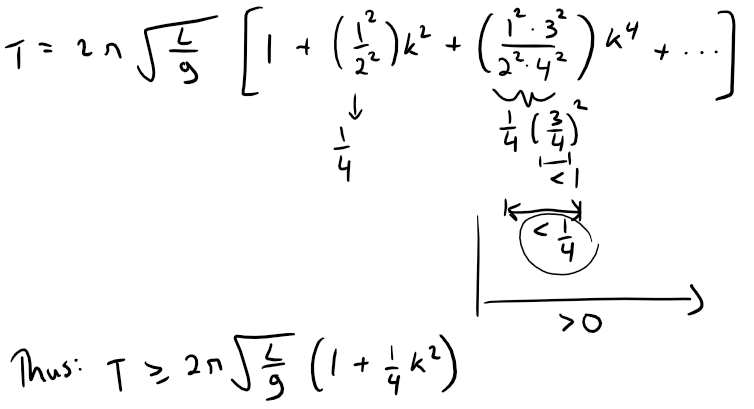
For the second inequality, first recall the geometric series from my earlier video:
https://peakd.com/@mes/infinite-series-definition-examples-geometric-series-harmonics-series-telescoping-sum-more
Retrieved: 6 August 2020
Archive: https://archive.vn/wip/Tr7ji
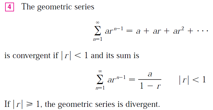
We can compare our Taylor series with the following geometric series:
(c) We substitute L = 1, g = 9.8, and k = sin(θ0/2) = sin(10/2) = 0.08716, and the inequality from part (b) becomes:
2 * pi * sqrt(1/9.8) * (1 + 1/4 * 0.08716^2) = 2.01090
2 * pi * sqrt(1/9.8) * (4-3 * 0.08716^2)/(4-4 * 0.08716^2) = 2.01093
2.01090 ≤ T ≤ 2.01093
So, T ≈ 2.0109
The estimate T ≈ 2 * pi * sqrt(1/9.8) = 2.0071 differs by:
(2.0109 - 2.0071)/2.0071 * 100 = 0.1893 % ≈ 0.2 %
If θ0 = 42°, then k = sin(42/2) = 0.35837 and the inequality becomes:
2 * pi * sqrt(1/9.8) * (1 + 1/4 * 0.35837^2) = 2.07153
2 * pi * sqrt(1/9.8) * (4-3 * 0.35837^2)/(4-4 * 0.35837^2) = 2.08103
2.07153 ≤ T ≤ 2.08103
So, T ≈ (2.07153 + 2.08103)/2 = 2.0763.
The one-term estimate is the same, T ≈ 2.0071, and the discrepancy between the two estimates increases to:
(2.0763 - 2.0071)/2.0071 * 100 = 3.4478 % ≈ 3.4 %
Exercise 6: Surveying
If a surveyor measures differences in elevation when making plans for a highway across a desert, corrections must be made for the curvature of the Earth.
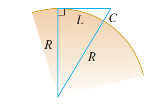
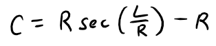
(a) If R is the radius of the Earth and L is the length of the highway, show that the correction is:
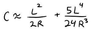
(b) Use a Taylor polynomial to show that:
(c) Compare the corrections given by the formulas in parts (a) and (b) for a highway that is 100 km long and take the radius of the Earth to be 6370 km.
Solution:
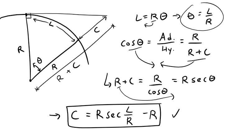
(a) L is the length of the arc subtended by the angle θ, so L = R θ by definition where θ is measured in radians.
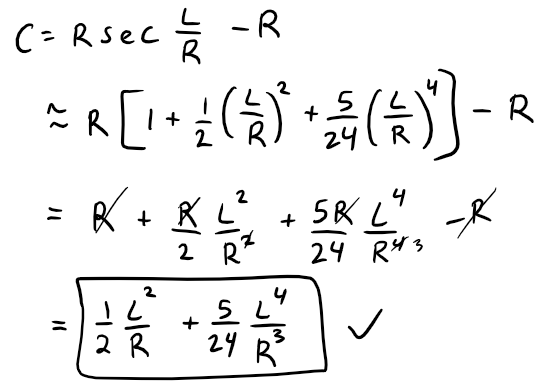
Thus we can determine the correction C as follows:
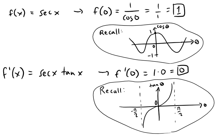
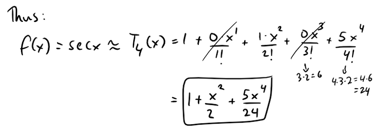
(b) First we'll find a Taylor polynomial T4(x) for f(x) = sec x at x = 0, that is to approximate small angle changes along the Earth.
Recall the basic trigonometric derivatives from my earlier videos:
https://peakd.com/hive-128780/@mes/trigonometry-derivative-of-sec-x-proof
Retrieved: 5 December 2020
Archive: https://archive.vn/wip/w06Ae
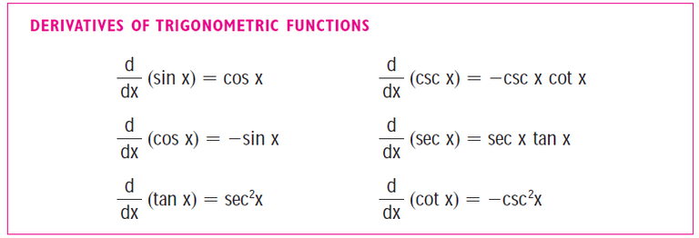
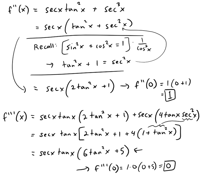
Now to determine the derivatives for the Taylor series:
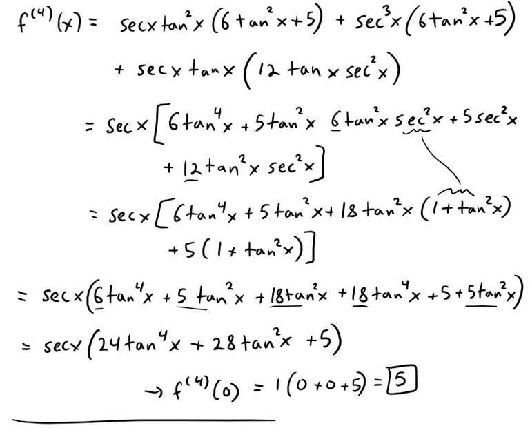
Now we can plug our approximation into the result from part (a):
(c) Taking L = 100 km and R = 6370 km, the formula in part (a) says that:
MES Note: The built-in OneNote calculator is in degrees by default and there isn't a secant function but there is a cosine function.
C = 6370 * 1/cos(100/6370 * 180/pi) - 6370 = 0.785 009 965 44 km
The formula in part (b) says that:
C ≈ 1/2 * 100^2/6370 + 5/24 * 100^4/6370^3 = 0.785 009 957 36 km
The difference between these two results is:
0.78500996544 - 0.78500995736 = 8.08E-9 km = 0.000 000 008 08 km
This is an accuracy of only 0.000 008 08 m or 0.00808 mm!