I. Introduction
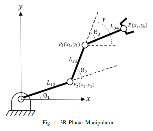
The mathematical modeling of the kinematics of a 3R planar manipulator involved in identifying the end-effector position or the joint angles. The 3R planar manipulator has three revolute joint and three links, as shown in Figure 1. The robot forward kinematics yields the end-effector position and its orientation from the given link lengths and joint angles. On the contrary, the robot inverse kinematics finds the joint angles from the given end-effector and its orientation.
The position of the robot end-effector is denoted by P as
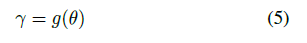
and its orientation relative to the world x-axis is denoted γ. The robot joint angles are denoted θi. The trigonometric functions, sine and cosine, are used extensively in the text so the following notations are introduced.
This notation is also extended to sums as
Link lengths are the distances between the joints and denoted as Lij , where i is the joint number closer to the base and j is the joint number to the end-effector. In this text, we derived equations for the forward and inverse kinematics of a 3R planar manipulator, in accordance to the earlier notations. Also, we create fkinematics and ikinematics functions in MATLAB for forward and inverse kinematics of 3R planar manipulator respectively, and evaluate it by comparing the result of each function.
II. METHODS
A. Forward Kinematics
The robot forward kinematics calculates the end-effector position and orientation given the joint angles and link lengths. The end-effector position is define by
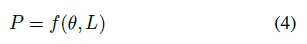
where θ comprises the joint angles and L is made up of all the link lengths. Also,
We derived the joint angles using the trigonometric relations in a right triangle. The joint positions are
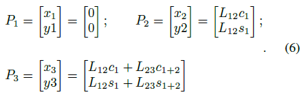
We take the vector sum of all the joint position and yield the forward kinematic equation for 3R planar manipulator as
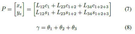
B. Reverse Kinematics
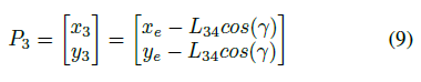
Robot reverse kinematics is a more useful study because the end-effector position is known. In reverse kinematics problem, the task is to find the joint angles given position p, orientation γ, and the link lengths. Initially, we solve the position of P3 and get
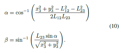
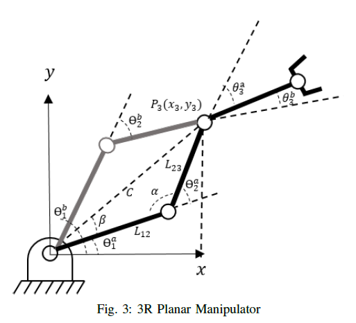
Hence P3 is obtained by equation 7, the joint angles θ1 and θ2 are given by a 2R inverse kinematics problem with P3 as the end-effector, as shown in Figure 3. We solve the angles α and β as
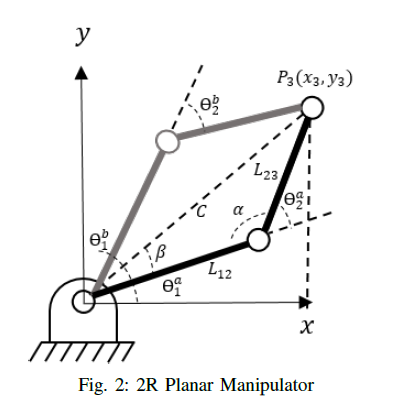
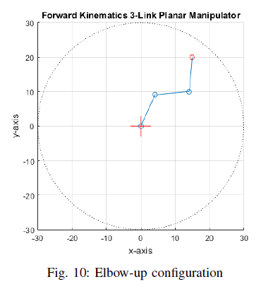
These angles are used to determine the joint angles θ1 and θ2. We keep in mind that there are two set of solution for the joint angles in 2R inverse kinematics problem. We refer joint 3 as the wrist, and joint 2 as the elbow. We compute the joint angles θ1 and θ2 by considering the elbow-up and elbow-down configuration, as shown in Figure 2, in reference to wrist angle θ3.
The joint angles θ1 and θ2 are
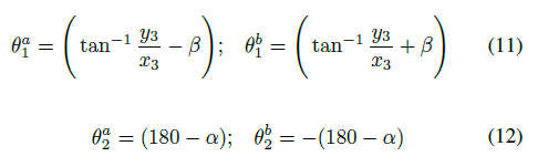
The wrist angles, θ3, are
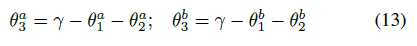
The a and b notation denotes the elbow-up and elbow-down configuration respectively. The joint and wrist angles are shown in Figure 3.
C. MATLAB Implementation
We implement the equations for the forward and inverse kinematics of a 3R planar manipulator in MATLAB. We create a fkinematics and ikinematics function for forward and inverse kinematics respectively. The fkinematics function accept the link lengths and the joint angles. It returns the end-effector position and orientation. Also, a plot of the 3R planar manipulator and its end-effector point is displayed. The script used for fkinematics is shown in listing 1.
function fkinematics(links1,links2,links3,theta1,theta2,theta3)
% Forward kinematics for 3-Link Planar Manipulator
% Inputs:
% links1,links2,links3 are length of each links in the robotic arm
% base is the length of base of the robotic arm
% theta1,theta2,theta3 are joint angles in reference to x-axis

format compact
format short

L12 = links1;
L23 = links2;
L34 = links3;
J1 = theta1;
J2 = theta2;
J3 = theta3;

%joint equation
x2 = L12*cosd(J1);
x3 = L23*cosd(J1+J2)+ x2;
xe = L34*cosd(J1+J2+J3) + x3;
y2 = L12*sind(J1);
y3 = L23*sind(J1+J2)+ y2;
ye = L34*sind(J1+J2+J3) + y3;
gamma = J1+J2+J3;
fprintf('The position of the end-effector is (%f, %f) and orientation is(%f)\n',xe,ye,gamma)

%plotting the links
r = L12 + L23 + L34;
daspect([1,1,1])
rectangle('Position',[-r,-r,2*r,2*r],'Curvature',[1,1],...
    'LineStyle',':')
hold on
axis([-r r -r r])
line([0 x2], [0 y2])
line([x2 x3],[y2 y3])
line([x3 xe],[y3 ye])
line([0 0], [-r/10 r/10], 'Color', 'r')
line([-r/10 r/10], [0 0], 'Color', 'r')
hold on
plot([0 x2 x3],[0 y2 y3],'o')
plot([xe],[ye],'o','Color','r')
grid on
xlabel('x-axis')
ylabel('y-axis')
title('Forward Kinematics 3-Link Planar Manipulator')
end
We set the link lengths, the end-effector position, and orientation as the input for the ikinematics function. The function returns the joint angles and a plot showing the 3R planar manipulator. Hence the inverse cosine yields to either a real or complex value, we set a conditional statement in the script so that inverse cosine would return a real-valued angle. The script used for ikinematics is shown in listing 2.
function ikinematics(links1, links2, links3, positionx, positiony, gamma)
% Inverse kinematics for 3-Link Planar Manipulator
% Inputs:
% links1,links2,links3 are length of each links in the robotic arm
% base is the length of base of the robotic arm
% positionx,positiony are joint angles in reference to x-axis
% gamma is the orientation

format compact
format short

L12 = links1;
L23 = links2;
L34 = links3;
xe = positionx;
ye = positiony;
g = gamma;

%position P3
x3 = xe-(L34*cosd(g));
y3 = ye-(L34*sind(g));
C = sqrt(x3^2 + y3^2);

if (L12+L23) > C
    %angle a and B
    a = acosd((L12^2 + L23^2 - C^2 )/(2*L12*L23));
    B = acosd((L12^2 + C^2 - L23^2 )/(2*L12*C));

    %joint angles elbow-down
    J1a = atan2d(y3,x3)-B;
    J2a = 180-a;
    J3a = g - J1a -J2a;

    %joint angles elbow-up
    J1b = atan2d(y3,x3)+B;
    J2b = -(180-a);
    J3b = g - J1b - J2b;

    fprintf('The joint 1, 2 and 3 angles are (%f,%f, %f) respectively for elbow-down configuration.\n',J1a,J2a,J3a)
    fprintf('The joint 1, 2 and 3 angles are (%f,%f, %f) respectively for elbow-up configuration.\n',J1b,J2b,J3b)
else
    disp('     Dimension error!')
    disp('     End-effecter is outside the workspace.')
    return
end
x2a = L12*cosd(J1a);
y2a = L12*sind(J1a);
x2b = L12*cosd(J1b);
y2b = L12*sind(J1b);
r = L12 + L23 + L34;
daspect([1,1,1])
rectangle('Position',[-r,-r,2*r,2*r],'Curvature',[1,1],...
    'LineStyle',':')
line([0 x2a], [0 y2a],'Color','b')
line([x2a x3], [y2a y3],'Color','b')
line([x3 xe], [y3 ye],'Color','b')
line([0 x2b], [0 y2b],'Color','g','LineStyle','--')
line([x2b x3], [y2b y3],'Color','g','LineStyle','--')
line([x3 xe], [y3 ye],'Color','b','LineStyle','--')
%line([0 xe], [0 ye],'Color','r')
line([0 0], [-r/10 r/10], 'Color', 'r')
line([-r/10 r/10], [0 0], 'Color', 'r')
hold on
plot([0 x2a x3],[0 y2a y3],'o','Color','b')
plot([x2b],[y2b],'o','Color','g')
plot([xe],[ye],'o', 'Color', 'r')
grid on
xlabel('x-axis')
ylabel('y-axis')
title('Inverse Kinematics 3-Links Planar Manipulator')
end
III. Result and Discussion
A. Forward Kinematics
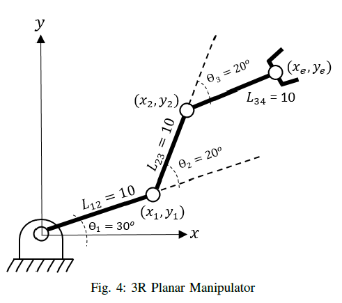
In this section, we evaluate the forward and inverse kinematics equations of a 3R planar manipulator. We substitute the values shown in Figure 4 in the fkinematics. In the Matlab window console, we run
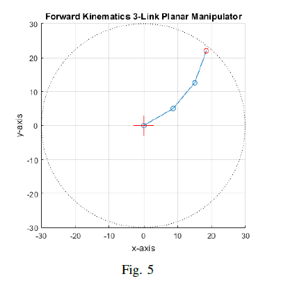
fkinematics(10,10,10,30,20,20)
and yield to the end-effector position, (xe = 18.508332, ye = 22.057371) and orientation, (γ = 70.00). Figure 5 shows the 3R planar manipulator.
The end-effector position and its orientation from the fkinematics is set as an input to ikinematics to evaluate it. The function must yield the joint angles shown in Figure 4. We run
ikinematics(10,10,10,18.508332,22.057371,70)
and we yield the following joint angles for elbow-down configuration are θ1 = 30.000009, θ2 = 19.999981, and θ3 = 20.000009. Hence the inverse kinematics has two set of unique solution, we have the joint angles for elbow-up configuration as θ1 = 49.999991, θ2 = −19.999981, and θ3 = 39.999991.
Thus, we verified that the forward kinematics equations which yields to a correct end-effector position and its orientation.
B. Inverse Kinematics
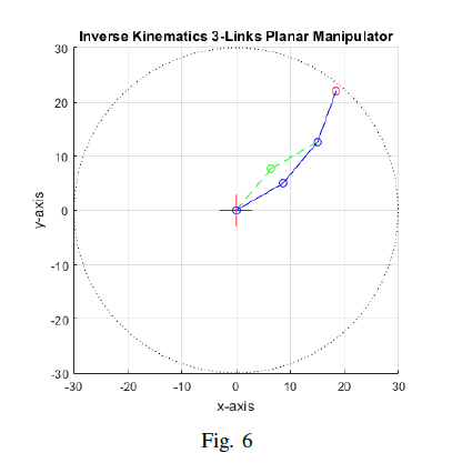
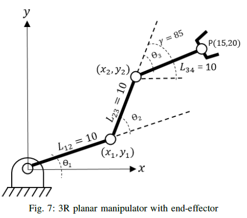
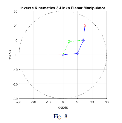
Figure 7 shows a 3R planar manipulator with an identified end-effector position and its orientation. We use ikinematics function in MATLAB to generate the joint angles. Then, we evaluate the result by substituting it as an input to fkinematics function. In the Matlab window console, we run
ikinematics(10,10,10,15,20,85)
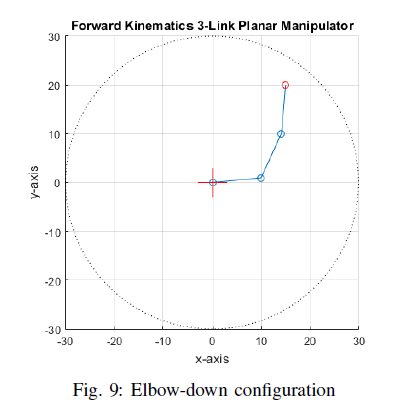
and yield a joint angle for elbow-down configuration as θ1 = 5.455370, θ 2 = 59.875741, θ3 = 19.668889 while for elbow-up configuration as θ1 = 65.331111, θ2 = −59.875741, θ3 = 79.544630. Figure 9 shows the 3R planar manipulator plot for the end-effector position xe = 15, ye = 20 and its orientation, γ = 85.
We validate the result by substituting the values to fkinematics and in Matlab console, run
fkinematics(10,10,10,5.455,59.876,19.669)
This gives us an end-effector position equal to xe = 15.000024 and ye = 19.999928, and orientation equal to γ = 85. The joint angles in elbow-up configuration also yield to the same end-effector and orientation.
Thus, we verified that the inverse kinematics equations which yields to the joint angles.
IV. Conclusion
In this text, we modelled the equations for the forward and inverse kinematics of a 3R planar manipulator as shown in Figure 1. In MATLAB, we wrote a script for the fkinematics and fkinematics functions. These functions are used to validate the forward and invers kinematics model in the text. The fkinematics function returns the end-effector position P and its orientation γ. The result of fkinematics is validate by using its result as an input to ikinematics function. On the contrary, the ikinematics function returns the join angles θ1, θ2 and θ3. We cross-validate the joint angles by setting it as an input to the fkinematic function.
Thus, the forward and inverse kinematics model yield to correct values for the end-effector position and its orientation, and the joint angles. Also, the joint angles, either elbow-up and elbow-down configuration, in the inverse kinematics model gives the same end-effector point and orientation when cross-validated.
V. References
[1] Lynch, K. and F. Park. “Modern Robotics: Mechanics, Planning, and Control.” (2017).
(Note: All images in the text are personally drawn by the author except those with citations. )
Posted with STEMGeeks
Posted with STEMGeeks
Thanks for your contribution to the STEMsocial community. Feel free to join us on discord to get to know the rest of us!
Please consider supporting our funding proposal, approving our witness (@stem.witness) or delegating to the @stemsocial account (for some ROI).
Please consider using the STEMsocial app app and including @stemsocial as a beneficiary to get a stronger support.