1. Introduction
Denavit–Hartenberg (DH) model is a kinematic model that relates the rotation and displacement of a reference frame B0 to the last link or end-effector frame Bn. The 4 × 4 homogeneous transformation matrix holds the rotation and the displacement matrix. The 3 × 3 rotation matrix defines the orientation of a joint or the end-effector while the 3 × 1 displacement matrix has the position of a joint or end-effector position.
In this paper, we modelled the forward kinematic of PUMA 560 robot manipulator using the DH model. In section 2, the derivation of the DH parameters and the homogeneous transformation matrices for each frames is discussed in details. In section 2.2, we implement a MATLAB script for the forward kinematics in section 2.1. Also, we evaluate the result by checking the rotation across the waist, shoulder and elbow joint to verify the correctness of forward kinematics in section 2.
2. Method
2.1 Denavit–Hartenberg (DH) Model
The DH parameters relates the rotation and displacement of frames Bn to Bn−1. The parameters are the joint angles θ, twist angle α, offset r, and link lengths d. The joint angle θ is the rotation at zn−1 to match the xn−1 to xn. The rotation at zn−1 includes all angular displacement at zn−1-axis. The joint angle at frame 1 is simply the angular displacement, θ1. This is true to all of the frames. In contrast, the twist angle α is the rotation at the xn to match the orientation of zn−1 to zn. For example, the twist angle α1 is −90◦ and it means that x1 rotates at −90◦ to match it with z0 to z1. All twist angles at each frames are defined by the earlier process.
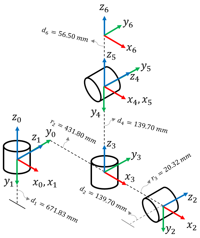
The offset r is the distance between the centers of n − 1 and n joints to the direction of xn. At frame 2, the offset r2 is equal to 431.80 mm. It denotes the distance at which the n-joint are displaced at xn as to n−1 joint. The link lengths d is the distance between the centers of n−1 and n joints to the direction of zn−1. In the figure, the link lengths d2 is equal to 139.70 mm hence it is the distance between n − 1 and n joint along z1. The DH parameters listed in Table 1 follows the earlier notation.
| Frame | θ | α | r | d |
|---|---|---|---|---|
| 1 | θ 1 | -90o | 0 | 671.83 mm |
| 2 | θ 2 | 0o | 431.80 mm | 139.70 mm |
| 3 | θ 3 | 90o | -20.32 mm | 0 |
| 4 | θ 4 | -90o | 0 | 431.80 mm |
| 5 | θ 5 | 90o | 0 | 0 |
| 6 | θ 6 | 0o | 0 | 56.50 mm |
The Denavit–Hartenberg (DH) model

is a standard kinematic model expressing position and orientation of a fixed coordinated frame relative to the nth−link or end-effector. The general homogeneous matrix Tn−1n consist the rotation and displacement vectors for a given joint angles. We define the homogeneous forward transformation matrix at each frame as
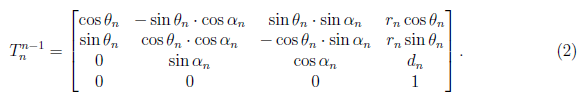
where the rotation matrix is
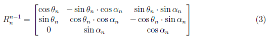
and displacement matrix is
Thus, the forward kinematic of PUMA 560 robot manipulator is given by the dot product of the forward transformation matrices at each frame. This is clearly establish in DH model. The position of the end-effector is in the displacement matrix d0n while its orientation is in the rotation matrix r0n.
2.2 MATLAB implementation
In this section, we create a script that implements the numerical solution for the forward kinematics problem of a PUMA 560 robot manipulator. We start with initializing the DH parameters listed in Table 1.
%DH parameters
J = [theta1 theta2 theta3 theta4 theta5 theta6]; %joint angles
A =  [-90 0 90 -90 90 0] ; %twist angle
r = [0 431.80 -20.32 0 0 0]; %offset as to xn
d = [671.83 139.70 0 431.80 0 56.50]; %offset as to z(n-1)
Next, we solve for the forward transformation matrices for all frames. This can be done by iterating equation 2 across all frames. The MATLAB scripts is shown in listing 2.
%Homogeneus Transformation
    for n = 1:6
        matT = [cosd(J(n)) -sind(J(n))*cosd(A(n)) ...
            sind(J(n))*sind(A(n)) r(n)*cosd(J(n));
            sind(J(n)) cosd(J(n))*cosd(A(n)) ...
            -cosd(J(n))*sind(A(n)) r(n)*sind(J(n));
            0 sind(A(n)) cosd(A(n)) d(n);
            0 0 0 1];
        T = [T; {matT}];
    end
Then, we solve for the orientation and positions of all joints by iterating equation 1 across all frames. We have the script as
%Joint Positions
    for i = 1:6
        if i == 1
            P = [P,{T{i}}];
        else
            matP = P{i-1}*T{i};
            P = [P, {matP}];
        end
    end
We create a fPUMA function comprising all the numerical solution and iteration that leads to the forward kinematics of a 6R PUMA 560 robot manipulator. We input to the function a set of joint angles and it results to the end-effector point and a three-dimensional plot of the robot manipulator links and rotation. After which, we evaluate the derive solution in section 2.1 by substituting the initial, boundary, and random conditions. This is to check if the analytical and computational solution in section 2.1 and 2.2 yield to a correct end-effector and plot from the input joint angles. The full script for the fPUMA function is shown in listing 4.
function fPUMA(theta1,theta2,theta3,theta4,theta5,theta6)
%input: joint angles at each frames
%ouput: end-effector position
%author: Jayson c. Jueco
format compact
format short
%DH parameters
J = [theta1 theta2 theta3 theta4 theta5 theta6]; %joint angles
A =  [-90 0 90 -90 90 0] ; %twist angle
r = [0 431.80 -20.32 0 0 0]; %offset as to xn
d = [671.83 139.70 0 431.80 0 56.50]; %offset as to z(n-1)
%forward kinematics
if J(1,1) >= -160 && J(1,1) <= 160 && J(1,2)>= -225 ...
        && J(1,2) <= 45 && J(1,3) >= -45 && J(1,3) <= 225 ...
        && J(1,4) >= -110 && J(1,4) <= 170 && J(1,5) >= -100 ...
        && J(1,5) <= 100 && J(1,6) >= -266 && J(1,6) <= 266
    T = [];
    %Homogeneus Transformation
    for n = 1:6
        matT = [cosd(J(n)) -sind(J(n))*cosd(A(n)) ...
            sind(J(n))*sind(A(n)) r(n)*cosd(J(n));
            sind(J(n)) cosd(J(n))*cosd(A(n)) ...
            -cosd(J(n))*sind(A(n)) r(n)*sind(J(n));
            0 sind(A(n)) cosd(A(n)) d(n);
            0 0 0 1];
        T = [T; {matT}];
    end
    P = [];
    %Joint Positions
    for i = 1:6
        if i == 1
            P = [P,{T{i}}];
        else
            matP = P{i-1}*T{i};
            P = [P, {matP}];
        end
    end
    %plotting the joint positions
    x = [0 P{1}(1,4) P{1}(1,4) P{2}(1,4) ...
        P{3}(1,4) P{4}(1,4) P{5}(1,4) P{6}(1,4)];
    y = [0 P{1}(2,4) P{2}(2,4) P{2}(2,4) ...
        P{3}(2,4) P{4}(2,4) P{5}(2,4) P{6}(2,4)];
    z = [0 P{1}(3,4) P{1}(3,4) P{2}(3,4) ...
        P{3}(3,4) P{4}(3,4) P{5}(3,4) P{6}(3,4)];
    hold on
    grid on
    rotate3d on
    plot3([x(1) x(2)],[y(1) y(2)],[z(1) z(2)]...
        ,'Color','b','LineWidth',5)
    plot3([x(2) x(3)],[y(2) y(3)],[z(2) z(3)]...
        ,'Color','r','LineWidth',5)
    plot3([x(3) x(4)],[y(3) y(4)],[z(3) z(4)]...
        ,'Color','g','LineWidth',5)
    plot3([x(4) x(5)],[y(4) y(5)],[z(4) z(5)]...
        ,'Color','c','LineWidth',5)
    plot3([x(5) x(6)],[y(5) y(6)],[z(5) z(6)]...
        ,'Color','m','LineWidth',5)
    plot3([x(6) x(7)],[y(6) y(7)],[z(6) z(7)]...
        ,'Color','y','LineWidth',5)
    plot3([x(7) x(8)],[y(7) y(8)],[z(7) z(8)]...
        ,'Color','k','LineWidth',5)
    plot3(x,y,z,'o','Color','k')
    xlabel('x-axis')
    ylabel('y-axis')
    zlabel('z-axis')
    title('Forward Kinematics of PUMA 560 Manipulator (6DoF)')
    view(0,0)
    disp('The end-effector position is ')
    fprintf('at Px = %f, Py = %f, and Pz = %f'...
        ,P{6}(1,4),P{6}(2,4),P{6}(3,4));
    disp('  ')
    disp('The DH model is  ')
    disp(P{6})
else
    disp('Joint angle out of range');
end
end
3. Result
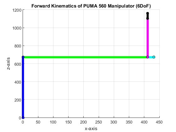
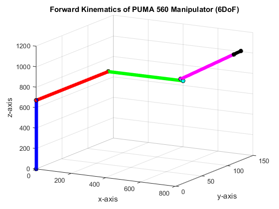
In this section, we present the result of the MATLAB implementation and validate the forward kinematics in section 2.1. Initially, we set the joint angles to zero and verify the end-effector is at the initial position shown in Figure 2.
At initial condition, the end-effector point is located at Px = 411.480000, Py = 139.700000, and Pz = 1160.130000. Figure 3 shows the plot indicating the orientation and position of each frames of the robot manipulator. The orientation of the forearm of robot is the same to the basis of the DH model in section 2.
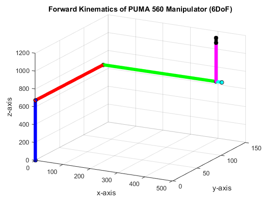
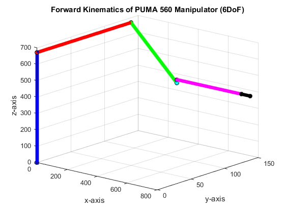
Next, we checked the rotation of the elbow and the shoulder joints by setting its respective angles to 45◦. These joints must have the same plane rotation to have a correct response. When we set joint angle θ2 to 45◦, we observed that it rotates along the x-z plane, as shown in Figure 4a. The end-effector is located at Px = 636.240540, Py = 139.700000, and Pz = 726.149943 for joint angle θ2 at 45◦ while the other joints at zero. For joint angle θ3, we set it at 45◦ while all other joint to zero. This result to an end-effector point located at Px= 636.240540, Py = 139.700000, and Pz = 726.149943. In Figure 4b, we observed that the elbow joint rotate in the x-z plane.
As stated earlier, the shoulder and elbow joint have the same rotation plane to yield a correct end-effector. Figures 4a and 4b indicate that the shoulder and elbow joint rotate in x-z plane. The results verifies the correctness of the kinematic equation in section 2. Furthermore, when we set the shoulder and elbow joint to 45◦ and other joint angles to zero, we observed the same plane rotation as shown in Figures 4a and 4b.
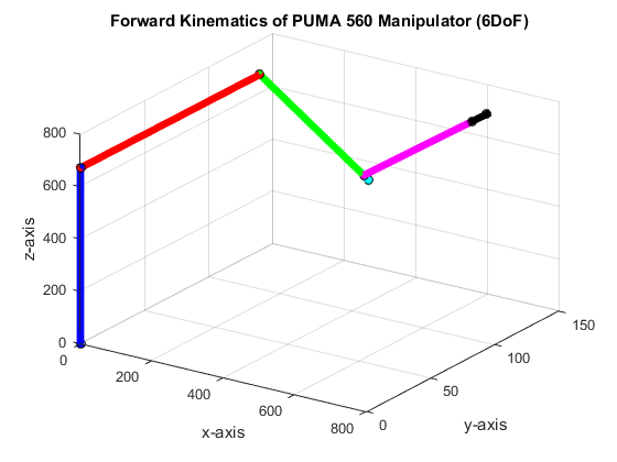
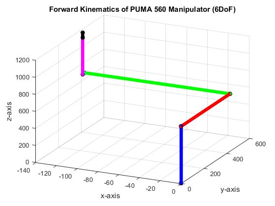
Then, we check the rotation of the waist joint. We set the joint angle (waist) θ1 to 90◦ and the other joint to zero. We observed that the waist rotate correctly, as shown in Figure 4d, in reference to the initial condition in Figure 3b. For a given set of joint rotation, we correctly locate the end-effector which was clear all throughout the plots in this section.
4. Conclusion
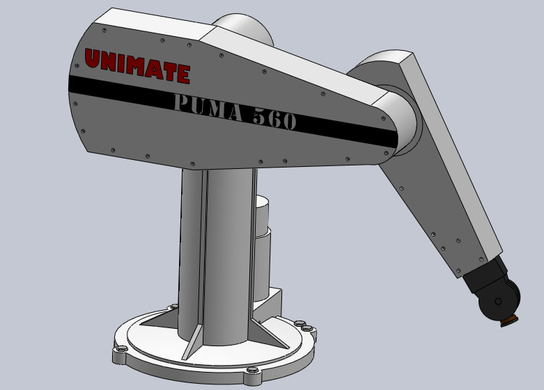
In this paper, we modelled the forward kinematics of PUMA 560 robot manipulator by using DH model. We established the DH parameters from the axes and joint representation for PUMA 560 robot manipulator as shown in Figure 2. We formed the homogeneous transformation matrices for each frames using the equations in section 2.1. The forward kinematic equations was implemented in MATLAB and evaluate the rotation across the joints. In section 3, we observed that the shoulder joint (joint1) and elbow joint (joint 2) rotate in the same plane. The result in section 3 verifies that the joint has correct rotation and response. Aside from checking the joint rotation, the end-effector is also verified. At initial condition (all joint angle θ equal to zero), the end-effector is at correct location as observed from the basis configuration in section 2. Thus, the kinematic equation taken from the DH model correctly gives the end-effector position and orientation.
5. References
[1] Lynch, K. and F. Park. “Modern Robotics: Mechanics, Planning, and Control.” (2017).
(Note: All images in the text are created by the author except for the 3D model in Figure 1. The 3D model is created by Gonzalo Loredo Neri and is free to download at grabcad.com)
Thanks for your contribution to the STEMsocial community. Feel free to join us on discord to get to know the rest of us!
Please consider supporting our funding proposal, approving our witness (@stem.witness) or delegating to the @stemsocial account (for some ROI).
Please consider using the STEMsocial app app and including @stemsocial as a beneficiary to get a stronger support.