1. Introduction
1.1 Descriptions of the System

The system consist of a voltage input, u(t), resistors, R1, R2 and R3, inductors, L1 and L2, and capacitors, C1 and C2. The current and voltages across each elements are shown in Figure 1. The output y(t) is equal to the voltage across the resistor, R2. The values of each elements are R1, R2, R3 = 10 Ω , L1, L2 = 0.5 H , and C1, C2 = 50 mF.
We apply mesh analysis to obtain the first-order differential equations:
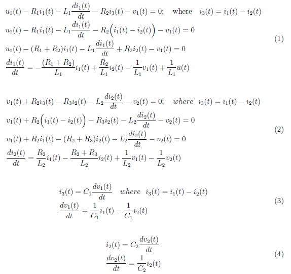
Then, we set the output equation as:
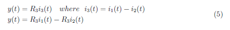
2. State Space Model
In this paper, we define the state variables
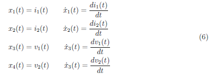
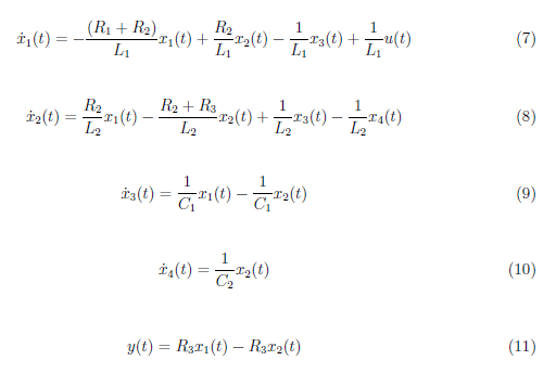
We replace the time-domain variables in the first-order differential equations (1− 5) with the state variables (6) to derive the state space equations of the system. We obtain the state space equations as
We derive the state space system representation from the equations (7−11). The state space system representation is defined by
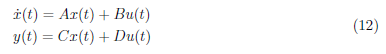
where A, B, C, and D are system, input, output, and feedforward matrices respectively. Then, we set the state space matrices as
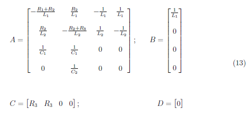
We substitute these state space matrices (13) to the equation in (12) to get the state space system representation as
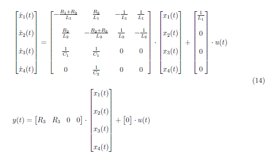
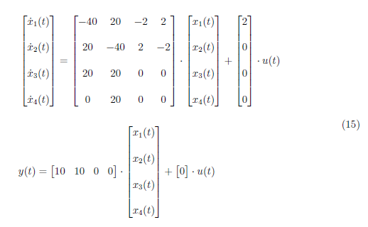
We obtain a state space model with numerical values by substituting the values of each circuit element in Section I. The state space model is defined as
3. Transfer Function
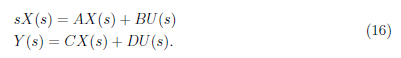
The transfer function G(s) is a ratio of output Y (s) and input U(s) of the system. We can derived the transfer function from the state space equation (12). Initially, we apply Laplace transform to the state space equation (12) and set the initial condition for system equal to zero. The state space equation in phase domain is defined as
We equate the equations in (16) and define the transfer function as
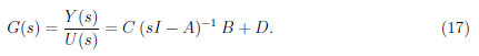
where I is an identity matrix.
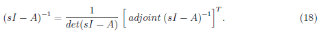
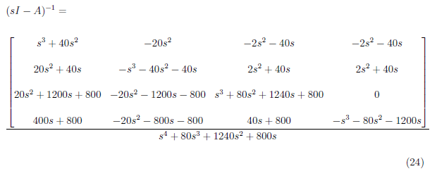
3.1 Solving the inverse of (sI-A)
The inverse of (sI − A) is defined by
Initially, we solve for the value of (sI − A) and get
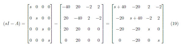
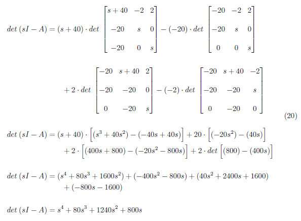
Next, we calculate the determinant of (sI − A) and acquire
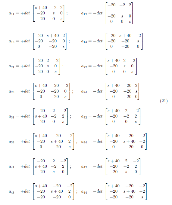
Then, we solve for the adjoint of (sI − A). We solve for each elements of the cofactor of (sI − A) by
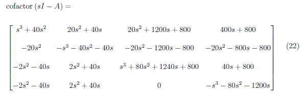
Solve for the determinants of the matrices in equation (21) and create the cofactor matrix of (sI − A). We defined the cofactor matrix of (sI − A) as
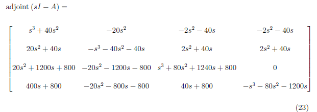
The adjoint of (sI − A) is the transpose of the cofactor matrix of (sI − A). The adjoint of (sI − A) is
Finally, the inverse of (sI − A) is
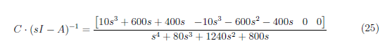
3.2 Solving the transfer function
We derived the transfer function of the system by substituting the values of C,(sI −A)−1, B and D to equation (17). First, take the dot product between matrices C and (sI −A)−1 and get
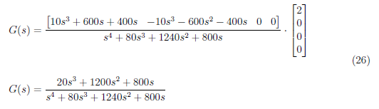
Then, take the dot product between equation (25) and B. The system’s transfer function is
3.3 Verify transfer function in MATLAB
The transfer function in equation (26) can be verified in MATLAB. We generate the states space system representation and its transfer function using the script:
%state spaace to transfer function
A = [-40 20 -2 2;20 -40 2 -2; 20 20 0 0; 0 20  0 0];
B = [2; 0; 0; 0];
C = [10 10 0 0];
D = [0];

%state space model
sys = ss(A, B, C, D, 0.25);

%transfer function
[num, den] = ss2tf(A, B, C, D);
The script result to state space model:
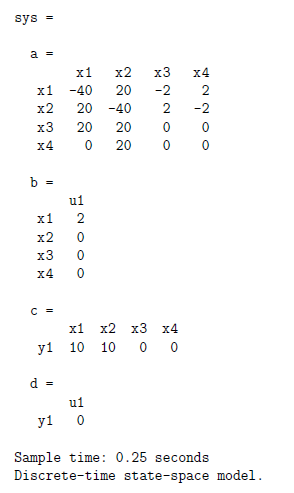
and the transfer function:
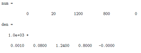
where num and den is the numerator and denominator of the transfer function.
5. Conclusion
In this paper, we are able to explain and derived the state space model the given system. We also derive the system’s transfer function by means of matrix and linear algebra. We verified the state space model using MATLAB. Thus, in the paper, we established the state space model of the given system and the system transfer function.
6. References
[1] Norman S. Nise. Control Systems Engineering (7th. ed.). 2015. John Wiley & Sons, Inc., USA.
[3] Bishop, Robert H., and Richard C. Dorf. "Modern control systems." (2017).
[4] Rowell, Derek. "State-space representation of LTI systems."
(Note: All image in the text is drawn by the author except those with attached citations.)
Posted with STEMGeeks