Gaussian Naïve Bayes
This post is short mathematical tutorial for understanding how naive bayes classifiers work. Hope you enjoy it!
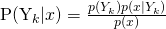
Let’s define a few terms. The first is Gaussian - also commonly called normal - which refers to the distribution of the values that we’re working with. The gaussian probability mass function (or what we’re generally just calling a distribution) might look like any any of these.

(Image is creative commons from Wikipedia)
where μ is the mean and σ is the variance (or squared standard deviation). The mean represents the location of the center, and the standard deviation is the spread of the distribution. When the mean is zero, and the standard deviation is 1, we call this a standard normal distribution. Generally, we can just call this a normal distribution, but if you want to impress people, be sure to say Gaussian. So this is the first large assumption we are making about the data - that is normally distributed. In reality, it might not really be, but as long as this approximation is good enough, we don’t really need to care - as long as we’re aware of our assumption.
The second necessarily defined term is Naïve Bayes - the naive refers to another assumption, and the bayes refers to bayes rule. The “naive” assumption says that each feature occurs independently, which is often not actually true. Once again, as long as this assumption works well in practice, we don’t really need to care about whether or not it true. So to unpack that, let’s introduce some notation. Let’s say that our target variable Y here is discrete (we are talking about a classifier) can take on k possible values  . Let’s also say that our inputs, X, or our data, is a table of sorts with columns
  where n is our number of columns. So this conditional independence assumption says that:

which says that each feature  is conditionally independent for every other feature
  for
for  , given our target
  . So in layman’s terms, this means that each feature is independent and doesn’t rely on the other features.
Secondly, Bayes refers to Bayes’ rule, which says that we can guess the probability of some class based on the conditional probability of the inputs. This takes the naive assumption and plugs it into bayes theorem:
which says that the probability of the target class given our input data is equal to the probability of the class, times the probability of the data given the class, all divided by the probability of the data. Since the denominator, the probability of the data, is the same across all classes, it can be thought of as a scaling factor and can often be ignored.
So, when we’re dealing with continuous data, we’re ultimately saying that the probability of seeing a particular value of this continue  can be derived from a normal distribution. So given a new input, say, some variable w we can calculate it by plugging it into this gaussian probability density function:
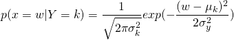
It’s if seeing math like that freaks you out - don’t worry! Its just a formula we plug stuff into and get values out of. Since its sort of annoying to write out, usually people write:
which is obviously a lot nicer to look at.
So by using bayes theorem, we can then calculate  for each value of k, and choose the class with the highest value. What makes this so awesome is that to build the classifier, we only actually need to the mean and the variance. How cool is that?
But what if our input data wasn’t continuous, but rather boolean? In that case, we just switch out the previous formula for a Bernoulli probability mass function rather than a gaussian probability mass function. So once again, given a new input, say some variable w, we can calculate it so:

where w must be either 1 or 0. Now we know how to calculate the probability of an input given a few assumptions about the values, which we call priors.
So to recap, Naive Bayes uses a two of assumptions:
- a distribution of the input values, e.g. Gaussian
- conditional independence of features (the “naive” part)
Then uses Bayes’ rule to figure out the probability. Part of what makes Naïve Bayes models useful is that these simple assumptions are easy to understand, explicit, and reduce the complexity of the model - which makes it quick to train and use.
Example
Let’s do this for real. Lets get some data - here we’ll try to use a gaussian naive bayes classifier to determine if a machine is likely to be used by malware as characterized by the bytes_received and bytes_sent. Each row represents a different host:
| used_by_malware | bytes_received | bytes_sent |
|---|---|---|
| yes | 170 | 85 |
| yes | 107 | 75 |
| yes | 108 | 76 |
| yes | 170 | 85 |
| no | 4620 | 1872 |
| yes | 8817 | 1331 |
| no | 4151 | 1758 |
| no | 6914 | 1265 |
| no | 538 | 733 |
| no | 3979 | 817 |
| no | 4028 | 801 |
| no | 538 | 740 |
| yes | 170 | 85 |
| yes | 170 | 85 |
| yes | 155 | 91 |
| no | 62 | 81 |
| no | 0 | 535 |
| yes | 90 | 94 |
| yes | 8352 | 2527 |
| yes | 7740 | 1755 |
…and lets say we have another 98,923 rows.
We already know that we only really need the mean and variance of each parameter:
| used_by_malware | mean_received | mean_sent | var_received | var_sent |
|---|---|---|---|---|
| no | 876.194707 | 583.119896 | 67628986.108950 | 1441638.354236 |
| yes | 3999.143071 | 1141.163828 | 323657959.129988 | 6862523.233360 |
So that is chill. So those compromise a total of 4 gaussians - each pair of mu and sigma can create a gaussian distribution.
However we also need to know the basic distribution of the classes, or in this case, the probability (given all the data) that a computer is used by malware.
| used by malware | count |
|---|---|
| no | 0.405971 |
| yes | 0.594029 |
We call these our “priors”. The decision to use these as priors seems reasonable to me, but the art and science behind choosing priors is beyond the scope of this piece. So now we have all our necessary variables to plug in !
Let’s pretend we just got a new host, and calculated the bytes received and bytes sent:
| used by malware | bytes_received | bytes_sent |
|---|---|---|
| ??? | 1012 | 800 |
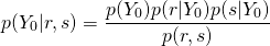
What we want to calculate is called our posterior.
Since our target variable is boolean, we really only need to choose one to calculate, since the other can be derived from our answer (by subtracting from 1). Let’s say used by malware = yes is  and used by malware = no is
  . We’ll call bytes_received r and bytes_sent as s:
however, since the denominator, also called evidence is going to be the same (a normalizing constant) on both classes  , we don’t actually have to calculate it[1].
So for just one of those terms,  :
:

Then we do the same calculation, for each of 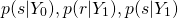 , plug those into the formula, after which we can determine which is larger, either
  (the probability of not having malware, given our inputs), or
  (the probaility of having malware, given our inputs). Whichever value is larger is our prediction.
which ultimately predicts that the data point does not represent a computer used by malware.
Conclusion
Naïve bayes makes assumptions - and those assumptions help make it:
- simple
- efficient
Something else that makes it useful is that it is well defined in cases of missing data points, where training or testing points are just not observed.
LaTex was generated via quicklatex. Thanks to @dkmathstats for pointing it out to me :)
If for some reason we had to, it is equal to: evidence =
 ↩
↩
This post reminds me to brush up on the Bayesian side of statistics. I am familiar with normal distributions, frequentist stats, stochastic calculus/processes but my Bayesian knowledge needs work!
For your data, are you using R/Python?
Thank you for the mention at the end for QuickLaTeX. It is a useful website.
Bayesian approaches are important! My knowledge needs work too :)
I do most of my work in python usually, but you can checkout the dataset I used here: https://gist.github.com/anonymous/8cab9745ad3b46fad388ca9d16099886
Great stuff, love that you show us the math!
Congratulations @metasyn! You have received a personal award!
Click on the badge to view your Board of Honor.
Do not miss the last post from @steemitboard:
SteemitBoard World Cup Contest - Home stretch to the finals. Do not miss them!
Participate in the SteemitBoard World Cup Contest!
Collect World Cup badges and win free SBD
Support the Gold Sponsors of the contest: @good-karma and @lukestokes
I have a problem with my naive bayes algorithme ( I'm starting to learn machine learning with scikit learn) I try to do give it numbers duo, usually 1 or -1 with a number and this represent a specific part out of 3 part and I want it to predict ( or calculate the probability) what part the combo will represent. Right now whatever I do the answer is always the first ( or 1 depending on your point of view). Do you have any advice/ ressource to read for a beginner?
Congratulations @metasyn! You received a personal award!
You can view your badges on your Steem Board and compare to others on the Steem Ranking
Vote for @Steemitboard as a witness to get one more award and increased upvotes!