In the previous chapter, the Abstract very briefly summarised the experiment and its outcomes. This chapter will introduce the relevant Physics behind this experiment, as well as low-temperature electron transport.

2 - Introduction

This section will be split into 2 main categories; the objectives of the experiment and the Physics behind resistivity.

2.1 - Objectives

By looking at how the resistivity of a material changes with varying temperature, some basic properties can be determined. In terms of a material’s electrical properties, they can be split into three groups: metals, semiconductors and insulators. Only metals and insulators have been analysed in this study.

2.1.1 - Metals

By taking resistance measurements of multiple Copper samples of varying thickness; the bulk resistivity, mean free path and Debye temperature could be determined.

2.1.2 - Alloys

The resistivity values of the alloy samples were experimentally calculated and studied, to understand how the different concentrations of Copper and Nickel within the alloy affected the resistivity.

2.1.3 - Kondo

Multiple Kondo samples, made up of Copper and Iron of unknown concentrations were also analysed for their resistivity-temperature dependence. From there, the concentrations were determined.

2.1.4 - Superconductors

For the Superconductors, multiple Niobium samples were tested in order to observe the special effect of Superconductivity. This was also achieved by looking at resistivity-temperature dependence.

2.2 - Resistivity

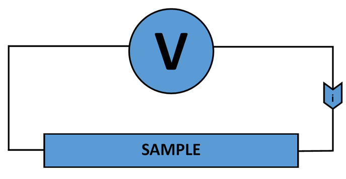
In order to measure the resistivity through a wire, the relation, ρ=RA/L can be used. To calculate a resistance, a current must be passed through a sample and its voltage must be recorded, as shown in figure 1.

Figure 1: Circuit set up to measure resistivity

The issue here, is that the measured potential difference also contains that of the lead and contact resistance. To measure the potential difference of just the wire, the 4 point probe method [1] is used, as shown in figure 2.

Figure 2: Circuit using the 4 point probe method

Any unwanted contact or lead resistance, in this method, is eliminated due to the driven current measuring the wire directly. If a DC current is used, thermal EMF becomes an issue. This can easily be eliminated by switching the current direction and finding the difference in the voltages; where this difference is the thermal, unwanted EMF. This 4 point probe method works well for wires, but when a sample is irregular-shaped, another method must be used. This method is called the Van der Pauw method and it is used to calculate the resistivity of objects that are not in the shape of a wire. Using this technique, 4 contact points are chosen around the edge of the sample; from this, two points are used to run a current through the sample and the other two measure the voltage, allowing for a resistance to be calculated. Figure 3, below, shows the contact points around the irregular-shaped sample.

Figure 3: Four points located around the irregular shaped sample

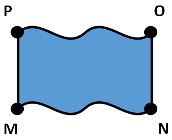
Once a resistance is calculated, the current is driven through the two points 90° to the previous configuration, for another resistance to be acquired. The following equation is then used to calculate the resistivity:

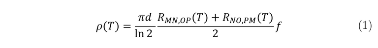
Where d= thickness of the sample and f= correction factor

Resistivity is a measure of how well a passing current is ’resisted’ from flowing through a material. Its origins arise from this flowing current interacting with phonons and impurities in the lattice of the specified material. Matthiesen’s rule explains this in terms of collision rates:

Electron-phonon scattering can be explained by the Bloch Gruneisen function [2]. Using the resistivity-temperature relation of a sample, a Bloch Gruneisen function can be fitted to give a range of useful values including Debye temperature and the mean free path of the material. The equation of the Bloch Gruneisen function is as follows:

Where ρ(0)= the impurity contribution to the resistivity and ρ_phonon= the phonon contribution to the resistivity.

ρ_phonon has an equation for itself, as shown below.

As can be seen from the integral, varying T_D in ρ_phonon gives relations ρ∝T and ρ∝T^5. The Fuchs Sondheimer relation is used to further study the effect of resistivity of a sample of varying thickness. The equation for the simplified Fuchs Sondheimer relation is [3]:

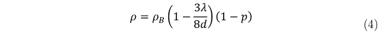
Where ρ_B= the bulk resistivity and p= the reflectivity ratio.

If you have any questions, leave them below and until next time, take care.

~ Mystifact

References:
[1]: http://iopscience.iop.org/article/10.1088/0953-8984/27/22/223201
[2]: https://link.springer.com/article/10.1007%2Fs11232-011-0003-4
[3]: http://www.qucosa.de/fileadmin/data/qucosa/

Please note; no copyright infringement is intended. All images used have been labelled for re-use on Google Images. If any artist or designer has any issues with any of the content used in this article, please don’t hesitate to contact me to correct the issue.

Previous LET chapters:
Chapter 1 - Abstract

Next chapter:
Chapter 3 - Experimental Techniques

Follow me on: Facebook, Twitter and Instagram, and be sure to subscribe to my website!

LET: Low-Temperature Electron Transport | Chapter 2 - Introduction