The Franck-Hertz experiment is probably one of the fundamental and important experiments in Quantum mechanics as it was the first experiment which clearly shows the quantum nature of atoms and the characteristics of Quantized Energy levels and transfer.

This is an incredibly important experiment and in this post I will be sharing the experiment I performed several years ago as an undergraduate so that you might be able to understand fundamentally how important the experiment was for the development of Quantum mechanics.
Franck-Hertz Experiment
1.) Objective
The primary objective of this experiment was to repeat a portion of the Franck-Hertz experiment, carried out in 1914 which demonstrates the quantization of energy transfer in non-elastic electron-atom collisions. In order to carry out this objective we were to measure the first excitation energy of mercury and hence develop a model that describes the excitation of mercury (Hg) and the energy lost by electrons via collisions causing the excitation of Hg.
2.) Introduction
The main purpose of this experiment is to repeat the Franck-Hertz experiment performed in 1914 and in order for us to completely understand what we are trying to reproduce, we must discuss the background theory and results of the 1914 experiment.
The Franck-Hertz experiment verifies that the atomic electron energy states are quantized by observing maxima and minima in transmission of electrons through mercury vapor. The variation in electron current is caused by inelastic electron scattering that excites the atomic electrons of mercury. The Franck-Hertz experiment confirms the Bohr Model of that atom. It was found that when electrons in a potential field were passed through mercury vapor they experienced an energy loss in distinct steps, and that that the mercury gave an emission line at λ = 254nm. This was due to collisions between the electrons and the mercury atoms.
The Franck-Hertz apparatus (shown in figure 4.1 in the apparatus section) consists of glass tube containing the circuitry. An electrode emits electrons when heated, which are attracted to a grid system by a driving potential across the glass tube. The grid consists of two layers, between which is the accelerating potential. Finally, there is a collector outside of the grid with a breaking voltage between them. As the accelerating potential is increased the collector current increases to a maximum until the electrons have enough energy to transfer to and excite the mercury atoms through collisions, which is E = 4.8eV (The first excited state of Hg). As such the collector current then drops off, as after collision less electrons are able to overcome the breaking voltage. As the accelerating potential is increased further the electrons can again excite the mercury atoms, and another maximum is found. This process is repeated. This relationship of minima and maxima in transmission of electrons is further discussed in the prediction of the model section. The general excitation-emission states relevant to this experiment are shown as a diagram below:

The figure above demonstrates the quantized excitation-emission states with relevant energies. With Energy required to excite to the next energy level being E = hf (Or shown in the diagram above as ΔE = hv).
For our case we can verify that the emission line of λ = 254nm will be produced from 4.9eV of energy as:
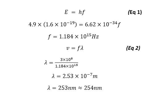
Nevertheless we will be showing that our energy is quantized in that each energy state showed as the minima/maxima of electron transmission from a plot of Anode current vs Accelerating voltage is 4.9eV apart, thus will prove the energy quantization of the first mercury state.
3.) Prediction of the model
We predicted before the experiment that a plot of anode current versus the accelerating voltage should look something like figure 2 below.
This plot shows the predicted collected anode current versus accelerating voltage, in which we can use to find the excited first energy state of mercury, it is given by the accelerating-voltage difference between 2 maxima, or the difference between 2 minima. We predict this curve based on the fact that we expect the energy states to be quantized (as this experiment has previously proven that it is), and we will be proving that this curve holds true, and building up a model to describe the excitation of mercury in the Franck-Hertz experiment later on in the results and data analysis section. We also predict that as a result of this curve that the first excitation state of mercury should be the difference in voltage between the minima of these ‘dips’ in collected current versus accelerating voltage, which we predicted to be 4.9eV between each ‘dip’ and as a result we expect the emission of 254nm of light (UV Spectrum) from our previous calculation.
4.) Procedure and apparatus
Before we get started with the results and data analysis, it is first important to discuss the procedure and apparatus that underpins the Franck-Hertz experiment. To setup our Franck-Hertz experiment we used a Franck-Hertz self-contained unit, a Franck-Hertz control box and an oscilloscope to read the data (anode current and accelerating voltage). A diagram of this setup is as below (Note this is a general setup and has been verified to be accurate to our setup however the image is not our setup but instead is a clearly set up Franck-Hertz experiment closely resembling ours)
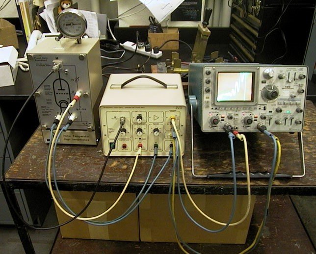
The box on the left is the Frack-Hertz apparatus where the excitation of mercury occurs within a tube inside, with the box (oven) temperature set at 180°C, which we found (during our exploration stage of the experiment) to be the point at which discernable dips of the anode current could be seen. The box in the middle is the Franck-Hertz control box, which the anode, cathode, grid and filament heat from the Franck-Hertz apparatus were plugged into, the control box would ramp an accelerating voltage through the apparatus and read the anode current. The data read from the control box, being the accelerating voltage and anode current were then output and read from the oscilloscope to be later output and analyzed using MATLAB.
An internal view of the Franck-Hertz apparatus is as below:
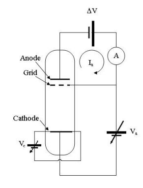
This shows the internal view of the Franck-Hertz tube, at which the breaking voltage is represented by ΔV , the accelerating voltage is applied between two layers of the grid, the cathode voltage and anode voltages are given by V_c and V_a respectively, the anode current (which we are to measure) is I_a measured by the ammeter A.
5.) Results and Data Analysis
We carried out the experiment and obtained data, and made sure to note any possible sources of error and uncertainty, which will be further discussed in the discussion section of the report. I will however note that the oscilloscope uncertainty is between 3% - 5%, so we will take the largest possible uncertainty as our uncertainty value for all of our oscilloscope data (Our Accelerating voltage and anode current will both have an uncertainty of at least 5%).
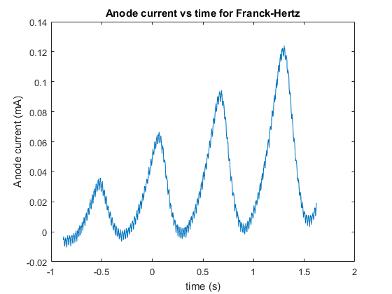
Our initial measurement with the oscilloscope yielded data that had a fair bit of hysteresis due to the resolution of the oscilloscope, we then used this to fine tune our measurement and obtain a new set of much better, and more accurate data which yielded a plot with less visible hysteresis, although some was still present due to the limitation of the oscilloscopes resolution. The data for this experiment is rather large, consisting of thousands of rows of data points, and hence the data will be posted to pastebin, with a link in the appendix. As stated previously the data from the first recording had a lot of hysteresis due to the resolution and hence we will not be reproducing plots or analyzing the low resolution data (as it will be less accurate and thus not have as much weighting to our final result). First we plotted anode current as a function of time in order to see if our Anode current as a function of time resembles the anode current versus the accelerating voltage, as accelerating voltage is just a linear ramp of change in voltage over time, thus the Anode current versus Accelerating voltage should just be a scaled version of the anode current versus time. And we can see from the figure below that it turns out that our Anode Current versus time does in fact look like our predicted Figure 2.
Next we plotted our anode current versus accelerating voltage, this plot is below:
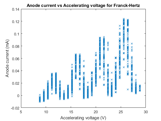
We can see from Figure 6 that our minima and maxima model of anode current from the excitation of mercury does in fact look like our predicted model, and predicted plot in figure 2, although the anode current values are significantly lower than Figure 2, though this is merely the amplitude of the excitation maxima and minima, determined by the filament temperature and hence can be altered without affecting the model and general plot.
From Figure 6 we used data cursors at the minima in order to calculate the voltage difference between the minima and hence the excitation energy between each point (We numbered these by serial number being the difference between two closest minima), we can also from Figure 6 that there is still a fair bit of Hysteresis, we could see that the minimum anode current was spread around a ‘range’ of accelerating voltage values and hence we took this to be the error in our voltage difference, which is the error in our electron volt excitation energy at each serial number. This error was caused mainly by oscilloscope resolution, but also from the 5% electronic error of the oscilloscope from a range of things including but not limited to the accuracy of analog digital conversion (Errors further discussed in the discussion).
The figure (with data cursors at the minima) is shown over the next page as Figure 7, we took the data points at the minima, as this is the minimum anode current read, which means that maximum mercury excitation occurs and hence we can use the difference between the accelerating voltage at two of these points to find the eV value for the excitation of mercury.
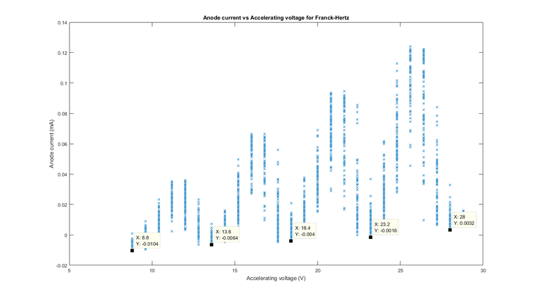
From this we can see that the difference between each minima is 4.8eV, we can see the ‘range’ of accelerating voltage values caused by the resolution error and uncertainty of our oscilloscope and was found using data cursors that around 0.8V around each voltage point had a very similar value to the minima, and hence we took this to be the uncertainty of our electron-volt value for the first excitation state of mercury at each serial number (where each serial number corresponds to a difference between two closest minima).
The only way to explain these minima/maxima dips is through quantum mechanics. Quantum mechanics tells us that the mercury atoms can only absorb certain quantized amounts of energy from the electrons. If an electron is moving too slowly when it bumps into a mercury atom, it cannot transfer any energy to it. However, if it gains enough speed, it will be able to transfer energy. So if our accelerating potential is chosen so that the electrons transfer all of their energy to mercury atoms right before they reach the grid, none of them will make it to the anode.
As we increase the potential further, the current will increase again for a while until it drops again. This time, the electrons transferred their energy to the mercury atoms halfway along their path and then once more right before the grid.
Next we plotted the difference in voltage, with error bars (for uncertainty) against the serial number, and as we can see from the plot above we will have 4 serial numbers in total, this plot can be seen in figure 8 below:

Normally one would plot these as data points and then do a linear fit to the data, but since our data was incredibly precise (all voltage difference values were 4.8eV), we simply plotted this as it is already a constant, straight line along the X-Axis, with equation: diff = 4.8. With diff being the difference between the dips. Hence from this plot we can conclude that the first excitation state of mercury is 4.8±0.8eV above the ground state. Although the error is fairly large (due to the resolution and intrinsic electronic error of the oscilloscope). The measured first excitation state here with the error, coincides with the predicted excitation energy of 4.9eV for mercury.
We also predicted a light emission wavelength of 254nm, using our result of 4.8eV we can see that the primary source of light emission will be at the wavelength of:
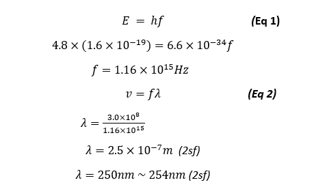
Our primary light emission is of the wavelength of 250nm which is quite accurate as it is very close to the actual predicted and theoretical value of 254nm, this means that this type of light emitted is part of the Ultra violet (UV) Spectrum and cannot be seen with the naked eye, however during the exploration part of our experiment, we were to increase the filament current to see the increasing amplitude of the anode current dips and in doing so we could also see a visible blue lines as shown in the figure below:

So why does this occur? Well the first excited mercury state produces UV light, which is invisible to a human eye or a camera. To make this picture, we had to make the tube and cathode far hotter than normal. This produced far more electron-mercury collisions than normal. So many, in fact, that some mercury atoms were excited into their second excited states. When the atoms decay from their second excited state to their first, they produce the blue lines seen in the picture.
6.) Discussion
We began this experiment with the prediction that our first excited state of mercury is 4.9eV above that of the ground state due to the predicted anode current versus accelerating voltage curve for the excitation of mercury. Due to the predicted 4.9eV to the first state from ground state, this means we predict that energy transfer is quantized and a discrete emission of light occurs (due to the energy-photon frequency relationship in equation 1) in our case with a wavelength of 254nm. Throughout our experiment we were able to determine that the first excitation state was 4.8±0.8eV above the ground state, the error in this was rather large due to the resolution of data obtained from our oscilloscope, and also due to the intrinsic electronic analog-digital conversion of data within the oscilloscope, as the oscilloscope was rated at 5% uncertainty with measurement data. Although we did not calculate 5% of the voltage, we can do that and see that 5% uncertainty of voltage difference would be:
Uncertainty(5%)=(0.05×13.6)-(0.05×8.8)
Uncertainty(5%)=0.24eV
This uncertainty is far smaller than the 0.8eV uncertainty in which we used, the other 0.56 comes from the resolution of our data and random error due to the small size of the measured anode current (hundredths of a milliamp) and in hind sight we should have used a larger filament current In order to increase this amplitude to reduce the amount of random error. As previously stated the uncertainty of 0.8eV was taken from the left and right points of the accelerating voltage at which the anode current was identical or incredibly close to the minima for a different voltage value. A plot with data cursors showing how we found this error is below:
.png)
Whilst this error is rather large, we did get a quite accurate value of first excited state energy of 4.8eV, which is very close to the theoretical value of 4.9eV and is thus accurate. All of our first-exited energy state values for each serial number were 4.8eV and hence our excited state data was precise, and thus our final set of data with its uncertainty is both precise and accurate for the first excited state energy from the ground state.
7.) Conclusion
The aim of this experiment was to repeat the portion of the Franck-Hertz Nobel Prize winning experiment in 1914 which demonstrates the quantization of energy transfer in non-elastic electron-atom collisions. This experiment had incredible significance (although unbeknownst to Franck and Hertz at the time) as it proved the Bohr model of the atom with quantized energies. The experiment was the first experiment to clearly show the quantum nature of atoms.
To repeat this experiment we used a Franck-Hertz pre-packaged apparatus, control box and oscilloscope. We took a few measurements to increase the resolution of data as far as possible and then took a final measurement of the anode current and accelerating voltage in order to find the quantized first energy state of mercury based on the difference in voltage between the dips of a plot of anode current versus accelerating voltage. We found the first excited energy state to be 4.8±0.8eV in which fits nicely with our predicted first energy state, the wavelength of photon emitted from this first energy state was then calculated to be 250nm which is accurate as it is reasonably close to the predicted theoretical value of 254nm light. We also found that blue light is emitted as the cathode current, or filament current increased this is due to the fact that more electrons are emitted at higher energies and hence mercury is therefore able to be excited to higher energy quantized states, such as the n = 2 state which emits blue light. To summarize, we conclude that our predictions were indeed correct for our excited first energy state and the wavelength of emitted light, however we also showed that higher energy states can be obtained with more collisions further demonstrating the quantization of energy states and their relevance to quantum mechanics and the bohr model of atomic energy states and spectra.
This is a great post! Nothing to add! :)
Join us on #steemSTEM / Follow our curation trail on Streemian
Thank you for this very interesting article. It has been advertised on our chat channel (and upvoted).
The steemSTEM project is a community-supported project aiming to increase the quality and the visibility of STEM (STEM is the acronym for Science, Technology, Engineering and Mathematics) articles on Steemit.
Good post !!
Clear and concise post, thanks.
Fine
hey @locikll I followed & upvoted u...please follow me on @farhanasayed & upvote my posts :)