Hi friends... @dexterdev is back with his Classical Molecular Dynamics Series. In case you missed my last article in this series, please see it here:
Classical Molecular Dynamics Series [Part - 4a]: Let us set up a simulation and run it!
Today we will simulate a small system which anyone can try out on their computer, provided you have installed NAMD and VMD. We will start from the psf and pdb file which we created in the last article using CHARMM-gui. I am linking those files here: step5_assembly.psf, step5_assembly.pdb
Let us keep things simple this time since we are simulating the system in laptop/desktop etc. Mine is an i7 processor, 8GB RAM machine. We will extract a single lipid from the above psf and pdb, add water and ions to it and then simulate it under 2 conditions.
- Condition 1: Temperature-273K
- Condition 2: Temperature-473K
(There are certain caveats here. High-temperature simulations are here to demonstrate the higher agitation in the molecules.)
Extracting a single lipid
Load VMD with $vmd step5_assembly.psf step5_assembly.pdb
Then load TCl-Console and type as below
set sel [atomselect 0 "resname DMPC and resid 1"]
$sel writepdb lipid.pdb
$sel writepsf lipid.psf
The above lines of code will pull out a lipid with resid 1 and write to a new psf and pdb file. For those who want to know more about DMPC phospholipid, please see my article on it here.
Adding water and ions to the system
Load the lipid.psf and lipid.pdb into VMD.
Go to Extensions -> Modeling -> Add Solvation Box.
Now give a suitable output name. I gave the name as lipid_solvate.
Now fill the all 6 min and max entries of Box padding with 10 (Angstroms is the unit.):
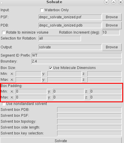
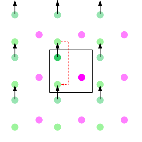
This will prevent the lipid's' interaction with its own image. Ooh... Now, what does that mean? Short answer: So we have simulations under periodic boundary conditions. Which means each box of the simulation system is repeated in the 3 dimensions. So the total charge in the system must be zero, else the charge won't converge.
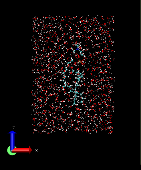
Once you press the Solvate button, a water box will be generated on top of lipid. Now we have to add ions to neutralize the system. This is pretty straightforward. Go to Extensions -> Modeling -> Add Ions. I chose NaCl with 0.15 mol/liter. Choose an out output name as in the solvation case. The name I selected is dmpc_solvate_ionized. So you have psf and pdb files corresponding to lipid in water and ions system.
The resultant system will look like below:
Simulation part
In the config file, you need to specify the periodic box size. To compute it you can use the Tcl script below:
get_cell.tl
proc get_cell {{molid top}} {
  set all [atomselect $molid all]
  set minmax [measure minmax $all]
  set vec [vecsub [lindex $minmax 1] [lindex $minmax 0]]
  puts "cellBasisVector1 [lindex $vec 0] 0 0"
  puts "cellBasisVector2 0 [lindex $vec 1] 0"
  puts "cellBasisVector3 0 0 [lindex $vec 2]"
  set center [measure center $all]
  puts "cellOrigin $center"
  $all delete
}
Load the above tcl script in Tcl-console after loading the psf and pdb file, by
source ./get_cell.tcl
get_cell
Let us start with config file for the 273K temperature case:
##############################################################
## JOB DESCRIPTION                                         ##
#############################################################

# 1 DMPC molecule in water and ions


#############################################################
## ADJUSTABLE PARAMETERS                                   ##
#############################################################

structure          ./dmpc_solvate_ionized.psf
coordinates        ./dmpc_solvate_ionized.pdb

set temperature    273
set outputname    DMPC

firsttimestep       0


#############################################################
## SIMULATION PARAMETERS                                   ##
#############################################################

# Input
paraTypeCharmm      on
parameters           ./par_water_ions.prm
parameters           ./par_all36_lipid.prm

temperature         $temperature

# Force-Field Parameters
exclude             scaled1-4
1-4scaling          1.0
cutoff              12.
switching           on
switchdist          10.
pairlistdist        15.0
margin               8.0

# Integrator Parameters
# fullElectFrequency*timestep <=4.0
# stable time steps:
#       with rigidBonds=all: electro:6fs;short-rangeNB:2fs;bonded:2fs
#       otherwise          :         2fs               2fs        1fs
timestep            2.0  ;# 2fs/step
rigidBonds         all  ;# Needed for 2fs steps
useSettle           on
nonbondedFreq       1
fullElectFrequency  2
stepspercycle       10
#########################
zeroMomentum        no
#########################


# Constant Temperature Control
langevin            off    ;# do langevin dynamics
langevinDamping     5     ;# damping coefficient (gamma) of 5/ps
langevinTemp        $temperature
langevinHydrogen    off    ;# don't couple langevin bath to hydrogens

#temperature coupling for temperature coupling
tCouple             on
tCoupleTemp         $temperature

if {1} {
# Periodic Boundary Conditions
# center of the periodic box; NOT ORIGIN!!!
# paste the output of get_cell.tcl here:
cellBasisVector1 29 0 0
cellBasisVector2 0 30 0
cellBasisVector3 0 0 41.5
cellOrigin -3.1667470932006836 -3.8784143924713135 10.219316482543945
}
wrapAll             on


# PME (for full-system periodic electrostatics)
# multiples of 2,3,5 & >=dimensions above
PME                 yes
PMEGridSizeX        30
PMEGridSizeY        30
PMEGridSizeZ        60


# Constant Pressure Control (variable volume)
useGroupPressure      yes ;# needed for rigidBonds
useFlexibleCell       no
useConstantArea       no

langevinPiston       on
langevinPistonTarget  1.01325 ;#  in bar -> 1 atm
langevinPistonPeriod  100.
langevinPistonDecay   50.
langevinPistonTemp    $temperature


# Output
outputName          $outputname

restartfreq         500000             ;# every 1 ns
dcdfreq             10000                ;#
xstFreq             10000
outputEnergies      10000
outputPressure      10000


#############################################################
## EXECUTION SCRIPT                                        ##
#############################################################

# Minimization
minimize            5000
reinitvels          $temperature

run 1000000 ;# for 2 ns
Assuming parameter files are in the current folder, open the terminal and type:
namd2 DMPC_NPT_eq.config > out. It took around 6 hours to finish the simulation(3109 atoms, 2ns simulation). After the simulation, you can load psf and dcd output to get the trajectory. Now you can repeat the entire simulation with a higher temperature by just replacing 273 to a higher number. The gif file in the top of the article shows two systems simulated as described.
It is quite obvious that the heated system fluctuates more vigorously. But we need to quantify it, right? In the next part, we will see more analysis related stuff.
Files
All input files and output files are uploaded in my github page for refreence. LINK TO FILES
References [Books for further reading]
Textbook references for learning theory of Molecular Dynamics:
- "Statistical Mechanics: Theory and Molecular Simulations" by Mark E. Tuckerman
- "Molecular Modelling: Principles and Applications" by Andrew R. Leach
- "Computer Simulation of Liquids" by D. J. Tildesley and M.P. Allen
References specific to NAMD and VMD:
CHARMM-gui related papers:
Join #steemSTEM
#steemSTEM is a community project with the goal to promote and support Science, Technology, Engineering and Mathematics related content and activities on the STEEM blockchain. If you wish to support the #steemSTEM project you can: Contribute STEM content using the #steemstem tag | Support steemstem authors | Join our curation trail | Join our Discord community | Delegate SP to steemstem
Convenient Delegation Links:
Follow me @dexterdev
 ____ _______  ______ _________ ____ ______
/  _ /  __\  \//__ __/  __/  __/  _ /  __/ \ |\
| | \|  \  \  /  / \ |  \ |  \/| | \|  \ | | //
| |_/|  /_ /  \  | | |  /_|    | |_/|  /_| \//
\____\____/__/\\ \_/ \____\_/\_\____\____\__/
By the way, this is a nice logo which @mathowl created for me. It is well suited for my MD series. :). Thank you @mathowl.

friend you are a great teacher, I think your dedication is amazing and admirable, I send you a hug full of successes
Thank you.
Real scientists doing real job... This is so real :D
Thanks man, great series, I hope some students will discover this
Thank you @alexs1320 :) steemit is motivating me to give out something unique. I believe we in steemit will produce more and more unique, original and helpful content for all. It seems that future is bright for the platform in general.
Good to be reading this from you. Unlike the somewhat pessimistic views you held before now. Good work btw
Yeah. I had pessimism. But now I started to think positively. :) Thankyou
Upvote for the "unique", non-Wiki posts!
So kick ass research :)
You are welcome :D. So what are the underlying equations that these numerical programs use?
The most underlying equation of any Classical MD program is 2nd law of Newton F=ma=-del(U), U represents the potential . I have touched upon those topics in the early parts of my series. But the numerical integrator has to take care of the symplectic property and reversible nature of equations.