In this post I’ll guide you through recurrent neural networks - to deep learning the other important part of machine learning. In a sense they also build a deep network, but the network goes deep in time that means that the input to the network must have some reasonable time dependent representation - examples to it are text (each character is assigned to different timestep in the sequence), videos, or also stock price development.
So, if the symbols in the sequence do not appear totally randomly - there are some underlying rules that determine what symbol can come next - then the network learns those rules and can predict what the next symbol will be.
It’s quite obvious how that would be useful for predicting the stock prices, but it is also very useful when creating a reliable reading system - even if you don’t have a perfect view of the next character you can quite well guess what it should be. We humans do it all the time, we never really read the whole words and our internal recurrent system just finishes it for us and the artificial (machine) recurrent systems try to mimic this behavior too.
And btw. Google just showed me how powerful their recurrent system is. I wrote stack prices by accident and it corrected me to stock prices - so obviously the system is also modelling pairs of words and not only checking if the word by itself is correct (exists). How cool!
Well let’s begin our journey to understanding of those powerful systems. Again I’m offering you some explanation and math that underlies the recurrent neural networks.
Basic recurrent neural networks
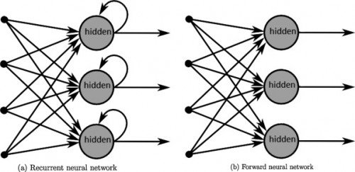
Recurrent neural networks (RNN) are a class of artificial neural networks that unlike feedforward neural networks have connections that form a directed cycle. The cyclic connections are called recurrent and they enable the RNN to hold the information from the past inputs for more than one time step. This enables the network to exhibit time-dependent behavior. This property makes RNNs useful for tasks involving prediction of sequences such as text recognition (printed and also handwritten), speech recognition, or natural language processing.
You can see it as if the network was sending itself information in time
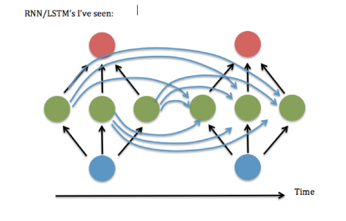
Courtesy of: http://stats.stackexchange.com/questions/210111/recurrent-neural-network-rnn-topology-why-always-fully-connected
... using a simple loop
And now to the math...
Standard recurrent neural network returns one output y_t at each time step

where W_hy is the hidden-to-output weight matrix and h_t is the output of the hidden layer at time t:

where the W_xh and W_hh are the weight matrices, W_xh is the input-to-hidden layer weight matrix, W_hh is the hidden-to-hidden layer weight matrix, the b term denotes the bias vector, and f is the activation function.
The problem with the basic RNN architecture is that the model can't learn longer sequences because of the vanishing gradient problem. The problem arises with the fact, that the errors computed in backpropagation are multiplied by each other every step of the propagation of error through time. If the gradient is small, the error diminishes towards zero, or on the contrary if it's very large the error goes beyond limits.
LSTM networks are very important. The main computational unit is a little bit more complicated, but the rest is just the same!
Long short-term memory network (LSTM)
The issue of the vanishing gradient was approached by Hochreiter and Schmidhuber in an alternative computational unit called long short-term memory (LSTM) (see figure). Its main distinction is the cell state within the LSTM unit which can remember an information for arbitrary long time. This way the LSTM can hold information theoretically throughout the whole presented history. LSTM units, however, don't suffer from the vanishing gradient problem because the activation function in the recurrency (in the cell state) is identity with the derivative of 1.0, which ensures that the gradient neither vanishes nor explodes. It remains constant and can be passed through the recurrent connection as many times as needed.
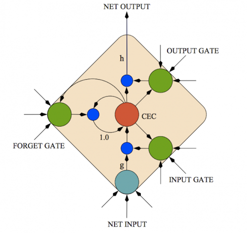
Courtesy of: http://haohanw.blogspot.cz/2015/01/lstm.html
The process of calculating the output from one LSTM unit is slightly more complex than in the case of the typical RNN neuron, however, it relies on the same principle. All LSTM units in hidden layer calculate their outputs h at time t. Those outputs are then used together with the new input data as the input to the units in time t+1. The equations for calculating h_t are as follows:
This is a little bit too much maths and too many equations, so if you don’t want to implement the LSTM unit by yourself you don’t really need to understand it.
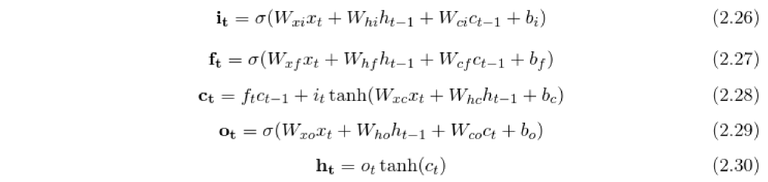
where i, f, o are respectively the input, forget and output gate vectors. The gates are either effectively blocking the information flow, if their output is close to 0, or letting the information through, if their output is close to 1. More precisely the forget gate decides if the cell state will forget the information it is retaining, the input gate decides if new information will be let in and the output gate decides if the information will be sent out of the LSTM unit. The c is the cell activation vector and h the hidden vector (the vector used for sending recurrent information). The W_xY is the weight matrix between input units and any of the gates, the W_hY is the weight matrix of recurrent connections from activations of hidden units to any gate and the W_cY is the weight matrix of recurrent connections from cell activations to any gate. The activation functions used in the model are sigmoid \sigma and hyperbolic tangent \tanh respectively.
And again learning of neural networks - the very same backpropagation but this time through time. But in principle it’s very simple, don’t worry.
Backpropagation through time (BPTT)
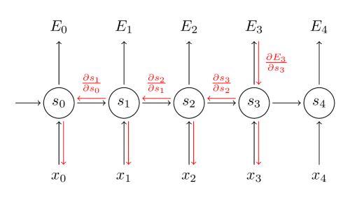
The most often used learning algorithm for recurrent networks is the backpropagation through time. It is a gradient-based technique for training recurrent neural networks. The basic idea works similarly to the backpropagation algorithm, however the error has to be propagated through the whole sequence back in the history (see figure below).
The BPTT algorithm begins with unfolding the recurrent neural network through time. Then the error is backpropagated not only through the feedforward connections, but also through the recurrent connections. The weights in the whole unfolded model are shared across the time, to achieve this, the gradients for input and recurrent weights are summed up at each time step and averaged into the final update for the weights.
The input, hidden and output weight matrix are in this section described as U, W, and V.
Denoting y_t as the output of the network and E_t as the error of this output at time step t the basic equation for the weight update in BPTT is calculated as following.
The goal is to calculate the gradients with respect to the U, V, W weight matrices. For the output weight matrix V the gradients are calculated similarly to standard backpropagation.
To calculate the weight deltas for the hidden matrix \Delta W the chain rule is applied

The output vector s_t of hidden layer at time t depends on the outputs at previous time steps which also subsequently depend on the parameters of the hidden weight matrix W. This recursive behavior leads to a different chain rule

where we sum up the contributions of activations at each time step to the gradient. As the matrix W is used in every time step up to the output at time step t, the gradients have to be backpropagated up to t=0.
The hidden weight deltas delta W are then equal to

The weight deltas for the input matrix U are calculated in the same way as for the hidden matrix W.
A few words for your comfort and fun
So I hope you enjoyed this post, or at least you didn't get bored too much. And if you finished it up to here - or scrolled down to here I have a reward for you. Here is a blogpost by Andrej Karpathy who is a researcher at Stanford and writes great posts about deep learning in general. This post is about recurrent neural networks, how they're so much fun and have great results. He also offers there his own code (I think it's in torch) that you can download and try for yourself.
Even if I don't understand the maths ...
Fantanstic i think we are at the beginning of a new era. The next year will be soo different than the past year and i am soo excited. Sorry for my english!
Well we'll see where this era will take us. There is a lot at stake and we must just hope that the scientists who're working on the (strong/general) artificial intelligence know what they're doing.
Hi, I am the new curator for @math-trail, a community dedicated to promoting the best articles on mathematics in its widest sense, including educational and cultural aspects.
I just upvoted your post - hope to see more in the future.
If you like to write about mathematics, then please follow @math-trail and I will follow you back and look forward to see fresh new content.
If you enjoy reading about mathematics, then please follow me so that you will receive the best content in your personal feed.
I am not a bot! Thanks!