What Will I Learn?
- You will learn about Weighted Voting Games
- You will learn what is Local Accuracy Estimates and when to use it.
Requirements
- Machine Learning
- Ensemble Learning Theory
Difficulty
Intermediate
Tutorial Contents
Ensemble learning is a machine learning paradigm where multiple learners are trained to solve the same problem. It draws inference from set of hypothesis instead of a single hypothesis from the training data. Ensemble learning is used very widely, because it can boost weak learners which predict slightly better than random guess to strong learners which can make accurate predictions.
Base learners solve the same problem, but they can be different from each other because of modelling techniques. population being studied and various other factors.
In practice, construction of very good ensembles is possible because statistically, when the training data available is too small, single classifier can easily select different hypothesis in the hypothesis space which gives the same accuracy on the same data. Therefore, the risk of choosing wrong classifier is high. Ensemble can take a cumulative decision and can reduce the risk of choosing wrong classifier.
Another reason why ensemble works is representational, by forming weighted sums of hypothesis in the considered finite hypothesis space, we can expand the hypothesis space and hence, it can provide a better approximation of the true hypothesis.
So, does that mean including many base learners in the ensemble will lead to better performance? The answer is no as experiments show that selecting a subset of base learners instead of using all also lead to better choice. The process of selecting optimal subsets of base learners among the available base learners is called ensemble pruning.
Classification Ensembles
In case of classification, majority voting is used to choose the ensemble prediction. In majority voting, each model makes a prediction and the output which receives more than half of the votes is chosen as the ensemble prediction.
This could be improved a lot, especially by assigning different weights to different voters (base learners) so that they influence the outcome of the ensemble. The weights can be assigned based on their competencies.
In case of binary classification, weights are calculated from the validation accuracy in the following manner.
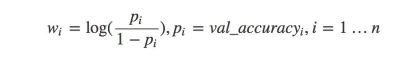
Weights are simply the log odds of the classifier validation accuracy. Let us numerically encode the classifier labels as 0 and 1. As this is binary classification setting, We just add weights corresponding to one class label. If it crosses a threshold, say half the times of summation of all the weights, then we elect that label. Keep in mind that weights of the classifier must be recalculated according to the class label chosen.
The main idea of local accuracy estimate is to change weights each time when a new test sample is taken instead of keeping it rigid. The weights are now depending on the conditional probability given test sample instead of validation accuracy.
To maximize the performance of the ensemble, we need to give more weight to that member which has highest accuracy in the neighborhood of the test point. This requires the classifiers to be independent which can be assured by performing bootstrap aggregation or the classifier can simply be assumed as independent.
The independence assumption is necessary to maintain the diversity of the ensemble. Moderate diversity is recommended for an efficient ensemble.
Now, let's check the performance of this algorithm on a simple 2 class classification dataset. Since the dataset is simple, very few training examples are needed. We knowingly train the individual classifiers on very few points to show how ensembles perform well.
First step is data preprocessing.
import pandas as pd
import numpy as np
columns = ['code_num','thickness','uofcsize','uofcshape','adhesion','secsize','bnuclei','chromatinb','nnucleoi','mitoses','output']
data = pd.read_csv('breast-cancer-wisconsin.data',names=columns)
data.drop(['code_num'],1,inplace=True)
data.replace('?',-99999, inplace=True)
data = data.astype(int)
X = np.array(data.drop(['output'], 1))
y = np.array(data['output'])
Second, we train 3 base learners, KNN, SVM and logistic regression on very few training points to satisfy the independent assumption.
from sklearn import preprocessing,neighbors,svm
from sklearn.model_selection import train_test_split
from sklearn.linear_model import LogisticRegression

X_train, X_test, y_train, y_test = train_test_split(X, y, test_size=0.9)
X_train, X_val, y_train, y_val = train_test_split(X_train, y_train, test_size=0.9)

clf1 = neighbors.KNeighborsClassifier()
clf2 = svm.SVC()
clf3 = LogisticRegression()

clf1.fit(X_train, y_train)
clf2.fit(X_train, y_train)
clf3.fit(X_train,y_train)

accuracy1 = clf1.score(X_test, y_test)
accuracy2 = clf2.score(X_test, y_test)
accuracy3 = clf3.score(X_test,y_test)
print(accuracy1,accuracy2,accuracy3)
#Out[2]: 0.652380952381 0.652380952381 0.703174603175
Next we define two utility functions, one which returns the log odd given the probability, another one returns the neighborhood of a test point in the validation data space.
def get_weights(p):
    p[p==1.0] = 0.99 #avoid inf error
    odds = (p)/(1-p)
    return np.log(odds)

from sklearn.neighbors import NearestNeighbors
neigh = NearestNeighbors(n_neighbors=3)
neigh.fit(X_val)

def get_local_weights(test_point,n_neigh):
    nearest_indices = neigh.kneighbors(test_point,n_neighbors=n_neigh,return_distance=False)[0]
    X_verify = X_val[nearest_indices]
    y_verify = y_val[nearest_indices]
    score_pred1 = clf1.score(X_verify,y_verify)
    score_pred2 = clf2.score(X_verify,y_verify)
    score_pred3 = clf3.score(X_verify,y_verify)
    acc_vector = np.array([score_pred1,score_pred2,score_pred3])
    weights=get_weights(acc_vector)
    return weights
Lastly, we write the code for weighted prediction function.
def get_weighted_prediction(sample_point):
    weights=get_local_weights(sample_point,4)
    prediction=np.array([clf1.predict([sample_point]),clf2.predict([sample_point]),clf3.predict([sample_point])])
    quota_weight = 0.0
    for _ in range(len(prediction)):
        if prediction[_] == 4:
            quota_weight = quota_weight + weights[_]
    if quota_weight >= np.average(weights):
        return 4
    else:
        return 2
So, let's check the gain in accuracy.
import warnings
warnings.filterwarnings('ignore')
ensemble_pred=[]
for _ in range(len(X_test)):
    ensemble_pred.append(get_weighted_prediction(X_test[_]))
ensemble_pred=np.array(ensemble_pred).reshape(y_test.shape)
from sklearn.metrics import accuracy_score
print(accuracy_score(y_test,ensemble_pred))
#Out[3]: 0.95873015873
That's some serious performance gain. Keep in mind that we trained these algorithms on very few training samples so, the performance gain from local accuracy estimates is really good.
Posted on Utopian.io - Rewarding Open Source Contributors
Your contribution cannot be approved because it does not follow the [Utopian Rules].
Hi, this is the reason your contribution was rejected
You can contact us on Discord.
[utopian-moderator]
@brobear1995, I like your contribution to open source project, so I upvote to support you.
This is fresh stuff! Thanks for writing.