After an intermezzo last week during which I introduced ideas about running a citizen science research project on Hive, it is now time to go back to normal blogs about particle physics and cosmology. Whereas the citizen science project will happen, I decided to keep my Monday blog as a regular slot for discussing particle physics. Another day will be selected for the citizen science project. This will be either Wednesday or Sunday, after accounting for the fact that Thursday is reserved for my write-ups in French.
Anyways… Two weeks ago I discussed in this blog how automated particle collider simulations could be achieved on regular computers. I tried to convey how complicated quantum field theory calculations could be achieved automatically, so that even a six-years-old child could deal with them without any problem.
The key idea is simple: those calculations can be seen as a recipe, so that it can be taught to a computer. As a consequence, it is sufficient to tell the computer which process we are interested in, what are the particle collider details and what is the model of physics (the Standard Model or anything beyond it) considered. I will come back to this in the first part of this blog.
Then I plan to continue this discussion, and explain how life is actually slightly more complicated because of the properties of the strong interaction, one of the three fundamental interactions. However, ‘complicated’ does not mean not programmable. Algorithms dealing with every single details of a particle collision in an automated manner therefore exist, preventing users from touching any single complication.
[Credits: Original image from the public domain (CC0)]
From quantum field theory to simulated (hard) collisions
In the previous blog, we focused on collisions of two highly-accelerated protons. The core process that is relevant in this case lies at the level of the constituents of the protons, and not at that of the protons themselves. At high energies, a proton can indeed be seen as a dynamical object made of constantly-interacting quarks (the most elementary building blocks of matter), antiquarks (their antiparticles belonging thus to the antimatter sector) and gluons (the mediators of the strong force). For more information about those fundamental particles, please consider having a look at this earlier post from December.
What thus matters in the present context is that a proton-proton collision such as those ongoing at CERN’s Large Hadron Collider is in fact a collision of quarks, antiquarks and gluons. The collision of two elementary particles among those then leads to the production of particles that could be either different from or similar to the initial ones. These produced particles could moreover be known particles (then we deal with a process of the Standard Model of particle physics), or even new particles beyond the Standard Model. Although any particle beyond the Standard Model is hypothetical, we are dealing with simulations so that we have the option to change the model of physics. In practice, this change is only limited by our imagination.
As said in the introduction to this blog, the goal is to simulate those collisions in a manner that is as realistic as possible. The first step relevant to this task is the simulation of the so-called hard process that is defined as follows. We begin by taking the two initial particles (one quark, antiquark or gluon for each proton) and then see how the theory considered allows us to produce a final state of interest.
Let’s be concrete for clarity reasons, and focus on a dedicated example: we consider the production, at the Large Hadron Collider, of a pair of particles comprising a top and an antitop quark. I recall that the top quark is the heaviest of all particles of the Standard Model, so that its study at hadronic colliders is very relevant as a test of the Standard Model and a window to new phenomena.
In order to simulate those collisions as they would occur in nature, we need to deal with a quantum field theory calculation. The idea of the present blog and of the previous one is to show how this can be automated on a computer. The starting point of our story is the master equation of the theory, from which we can extract the building blocks embedding the properties of any process. Those building blocks are given by a set of diagrams, the so-called Feynman rules of the model.
In the left part of the figure below I show what these Feynman rules are for the Standard Model.
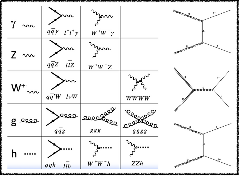
[Credits: @lemouth]
We can then use these building blocks to connect to connect the initial state and the final state of any process. If there is no way to connect them, then the process is forbidden. It there is one or more ways, then the process occurs. In the right part of the figure, I show all the dominant ‘connections’, or Feynman diagrams in our jargon, between an initial state made of two gluons and a final state made of one top quark and one antitop antiquark. Please try it by yourself and check whether other diagrams exist. Don’t hesitate to let me know if you find any.
While it may be cumbersome to get all diagrams for a given process, especially if there are many particles in the final state due to the growing combinatorics, this task is an easy one for a computer. Very efficient methods have thus been designed during the last decades, so that the issue of getting all diagrams associated with any given process of any specific model is considered as solved.
In a second step, the diagrams must be converted into an equation, that consists of a high-dimensional integral. This integral corresponds to a sum over all possible configurations of the final state. We indeed want to produce two top quarks (in our example), and we don’t really care whether they are produced back-to-back, they travel in the same direction, or carry a lot of or a little energy (and so on). We solely want to produce two top quarks at a hadronic collider, regardless of their behaviour.
This ‘diagram-to-integral conversion’ is again an easy task for a computer, as there is simply a recipe to follow. Algorithms therefore exist and this issue is also a solved one.
Finally, the integral has to be evaluated numerically. This generally relies on an adaptive integration procedure (for instance the VEGAS algorithm). The advantage of this method is that it explores all configurations of the final state and estimates how rare/frequent they are. From this, we can generate simulated collisions featuring configurations of the final state in agreement with their frequency of appearance, or equivalently as they would occur in nature.
This is where the story ended up last week. However, the production of two top quarks or any process like this one are actually very far from what we could observe in a detector. This is the topic of the second part of this post.
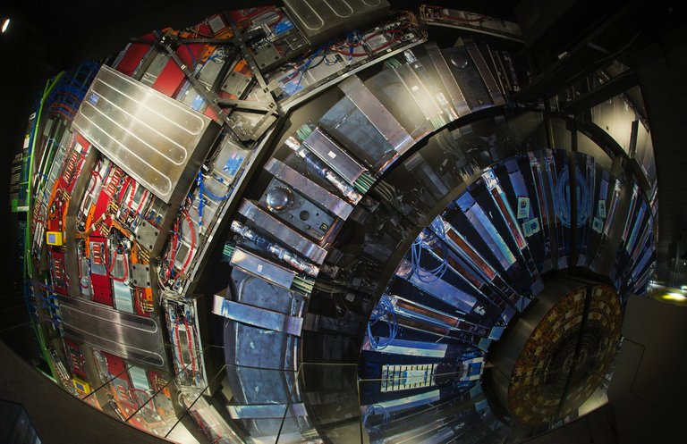
[Credits: Eric Bridier (CC BY-ND 2.0)]
From instability to stability
So far, we got interested in the production of any final state of interest in a collision such as those ongoing at the Large Hadron Collider. Whatever final state we pick, it however often comprises unstable massive particles, that decay after a very short amount of time. For instance, a top quark decays into a W boson and a b-quark in about 10-25 second (this amounts to 0.0000000000000000000000001 second). In a second step, the W boson produced in the top-quark decay also decays almost instantaneously in something like 10-25 second.
Those super small numbers teach us one thing. In general, any produced massive particle can be considered as instantaneously decaying. The reason is that the detector electronics is not capable to be that fast, and to measure that such a decay occurred after the initial process. In particular, this holds both for timing and position. From its perspective, the detector sees everything as emerging directly and instantaneously from the collision point.
We thus need to add heavy particle decays to the picture built so far. In order to do this, we need to understand how to get information on which particle decays into what, and with which probability. This is derived from the same master equation as the one used so far. All possibilities for the decays of a specific particle derive from what is achievable with the Feynman rules at our disposal.
This means that we can again make use of a computer algorithm to build the diagrams and extract the relevant equations. This proceeds quite similarly to what we described above. This implies that we can make use of a single numerical program that deals with the production of a full final state in which all particles are stable on detector scales. If there is an intermediate unstable particle like a top quark, then the code handles its decay and includes it in the simulation.
After including particle decays in simulations, we end up to simulate collisions in which the final-state products consist in muons, electrons, light quarks (up, down, strange, charm and bottom quarks), neutrinos, gluons and photons. In terms of a theoretical context beyond the Standard Model of particle physics, then we need to add any new particle that is stable to this list. For instance, any dark matter particle that would fly away from the collision point where it has been produced should be added to it.
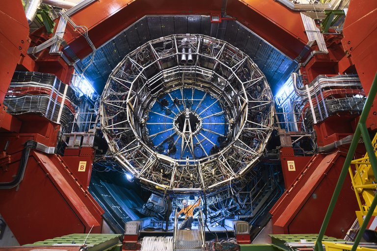
[Credits: CERN]
The strong interaction messing it up
The story however slightly gets more complicated…
In the list of stable final-state particles established in the previous section, we can notice the presence of quarks and gluons, two classes of particles sensitive to the strong interaction. In addition, the energy of all particles arising from a high-energy collision is, by definition, usually very large. We thus have a set of strongly-interacting and very energetic quarks and gluons in the final state. This has profound consequences, that mess up the clear picture we derived so far.
The properties of the strong interaction tell us that any accelerated (or equivalently highly-energetic) strongly-interacting object like a quark and a gluon radiates. The radiation process splits the radiating object (namely the mother particle) into two daughter particles that share the initial energy. The energy of each of the two daughters is thus smaller than that of the mother object. The radiation process hence allows for the energy of the produced quarks and gluons to decrease.
In order to get the structure of the radiation, we have to rely (once again) on quantum field theory. I won’t enter into details of calculations. I instead prefer to only indicate that radiation occurs generally in a collimated way, i.e. that the two produced particles in the radiation process are very close to each other. Moreover, the energy is in general very asymmetrically shared: one of the particles will be very soft (i.e. with a very small amount of energy) and the other one quite hard (i.e. with a large fraction of the available energy).
From this we can built a full radiation history. An initial energetic quark or gluon radiates, so that we end up with two objects with less energy. Those two objects then radiate other quarks and gluons, that then radiate, and so on. From one single energetic particle, we thus end up with a full cascade of very collimated quarks and gluons, each of them carrying a smaller amount of energy than their respective mother particle.
The above chain reaction is what we call parton showering. All produced quarks and gluons from the hard process end up being somewhat dressed with a lot of low-energy quarks and gluons.
This picture is illustrated on the figure below by everything that is in red. We can see a few particles on the left of the figure that radiate other particles, radiating themselves other particles, until the process stops (where the red turns green on the figure). The reason for this stop is simply the amount of energy, that has become too small for another radiation to occur.
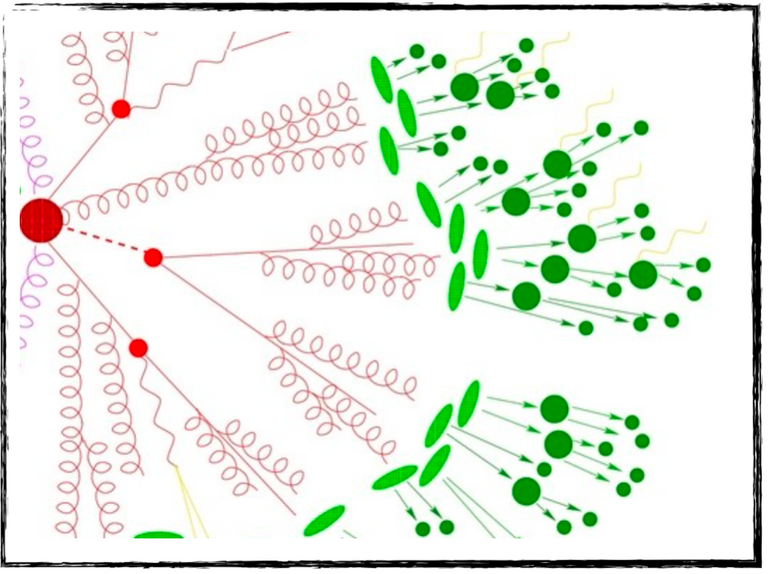
[Credits: A Sherpa artist (image available everywhere in the HEP community)]
The strong interaction is however not done with us. This can be seen from green parts in the above figure.
Those green blobs illustrate that the strong interaction… is strong. Free quarks and gluons do not exist as such in nature, and combine to form composite objects (that are generically called hadrons, as discussed in this earlier blog). In our jargon, we say that quarks and gluons confine. Particle physicists hence know the true meaning of confinement for many years… (I am wondering who will read that far).
These freshly-made hadrons are then very unstable, and decay into each other. Some of those decays are very quick, and others lead to some displacements. This is illustrated on the figure above. Any green blob is a hadron, and we can notice that heavier hadrons (big blobs) decay into lighter hadrons (small blobs).
Our initial collision has thus produced tons of hadrons, that interact further with a detector. Parton showering and hadronisation may seem rather complicated, but we have a few dedicated programs dealing with them.
A parton showering algorithm constructs the ‘cascade radiation history’ and relies on Markov chains, so that any specific emission is implemented independently of the previous ones. The related equation is an evolution equation dictated by the quantum theory of the strong interaction. This equation instructs us how a given quark or gluon radiates, and when this could occur as a function of its energy.
Hadronisation is a different story. Here, there is no master equation to be used and we must rely on phenomenological models not derived from first principles. However, they work well, and are moreover universal. This means that they can be used in the context of any collision process, regardless of what is happening at high energy (I recall that hadronisation consists of low-energy phenomena).
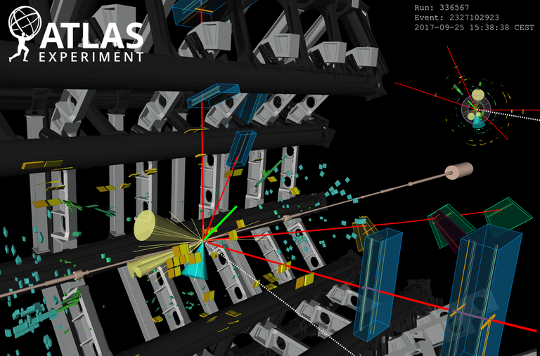
[Credits: CERN]
Take-home message: parton collider simulations in a nutshell
With this blog, I have tried to convey how particle collisions are simulated numerically. The full process is factorisable, so that dedicated codes have been designed to deal with specific parts of it.
We have codes that deal with (known or new) particle production at high-energy colliders, as well as with their decays. They rely on quantum field theory calculations, and on Feynman rules in particular. From there, other codes have been designed to deal with the simulation of the strongly-interacting environment inherent to a hadron collider such as CERN’s Large Hadron Collider. They include parton showering (radiation of strongly-interacting particles by other strongly-interacting particles) and hadronisation (formation of composite objects made of quarks and gluons).
From there, the story is almost over, but not quite. All those hadrons (as well as electrons, photons, muons that have not participated to parton showering and hadronisation) eventually interact with a detector, and leave tracks and energy deposits inside it. Physicists then need to reconstruct, from those tracks and deposits, what happened in a collision. After decades of experiments, we can probably say that this is bread and butter. Of course, we have dedicated computer programs to help.
I believe I should now stop writing, this blog being already quite dense. Feel free to ask for clarifications in the comment section if necessary. I would be very happy to answer.
This being said, I wish you all a very nice week!
This is a be good one and nice write,am seeing lot of idea coming from this
Thanks for passing by and the nice comment. I really like to put a lot of material all together in a blog, although I must admit that it may sometimes frighten any reader ;)
Thanks for supporting the author! !1UP
Save the best for last :)
What a day. Physics is a relief after today. My first question is simple and maybe silly:
The composite objects made up of free quarks and gluons are called hadrons. Is it a coincidence that the collider is called a Hadron collider?
When we do our computer simulations we are going to be looking for new particles? I followed much of the discussion pretty well. It will take a reread when I go to bed.
A couple of comments: your writing style does help the reader to get along:
:))
Also, the diagram (Sherpa artist) is very helpful. Very non-technical. Easy to understand. The Feynman rules for the Standard Model was a little tough. Really kind of skipped that (sorry) after giving it a try.
Thanks @lemouth for another amazing blog. I hope I can do this project. You say we have the formulas. Once we put them in the computer, the computer will do the work for us, I suppose.
Have a great week. Hard week ahead for me, but nothing to be done about that.
Thanks for passing by my blog and for the interesting questions. Sorry that you didn't get the Feynman rules, but I must admit that I was quite fast on this part.... This may deserve a full blog by themselves, one day... ;)
Absolutely not. Hadrons are particles made of quarks and gluons, and protons are just one example of hadrons.
This is precisely the point behind those computer codes. We indicate to the code in which processes we are interested, and the code does all calculations in the background for us.
Thanks for supporting the author! !1UP
amazing post friend
Thanks a lot for passing by!
Thanks for supporting the author! !1UP
The rewards earned on this comment will go directly to the person sharing the post on Twitter as long as they are registered with @poshtoken. Sign up at https://hiveposh.com.
Congratulations @lemouth! You have completed the following achievement on the Hive blockchain and have been rewarded with new badge(s):
Your next target is to reach 79000 upvotes.
Your next payout target is 34000 HP.
The unit is Hive Power equivalent because post and comment rewards can be split into HP and HBD
You can view your badges on your board and compare yourself to others in the Ranking
If you no longer want to receive notifications, reply to this comment with the word
STOPTo support your work, I also upvoted your post!
Check out the last post from @hivebuzz:
Thanks for your contribution to the STEMsocial community. Feel free to join us on discord to get to know the rest of us!
Please consider delegating to the @stemsocial account (85% of the curation rewards are returned).
You may also include @stemsocial as a beneficiary of the rewards of this post to get a stronger support.
Your content has been voted as a part of Encouragement program. Keep up the good work!
Use Ecency daily to boost your growth on platform!
Support Ecency
Vote for new Proposal
Delegate HP and earn more
Another great idea!
!1UP
You have received a 1UP from @ivarbjorn!
@stem-curator, @vyb-curator, @pob-curator, @neoxag-curator, @pal-curatorAnd they will bring !PIZZA 🍕
Learn more about our delegation service to earn daily rewards. Join the family on Discord.