1. Introduction

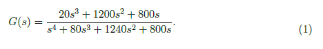
The system consist of a voltage input, u(t), resistors, R1, R2 and R3, inductors, L1 and L2, and capacitors, C1 and C2. The output y(t) is equal to the voltage across the resistor, R2. The values of each elements are R1, R2, R3 = 10 Ω, 1 , L2 = 0.5 H and C1, C2 = 50 mF. The system has a transfer function equal to
2. System Representation in Simulink
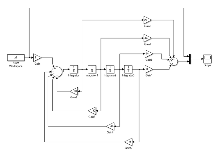
We represent the transfer function in equation (1) as a block diagram in Simulink, shown in Figure 2. The block diagram representation of the system consist of an input, a scope, a multiplexer, two summing point, three integrator, and ten gains. In MATLAB, we generate a chirp signal with a frequency between 0 to 10 Hz by using the script:
%system identification
t = 0:0.0001:30;
t1 = [0:0.0001:60]';
y = chirp(t,0,60,10);

x = wrev(y(1,1:end-1));
xa = [y x]';
x1 = [t1 xa];
plot(t1,xa);
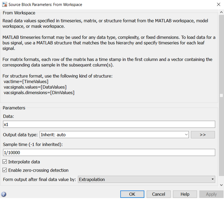
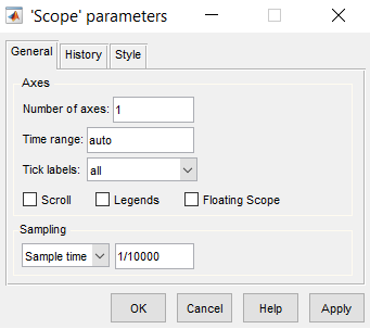
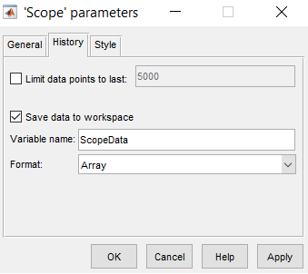
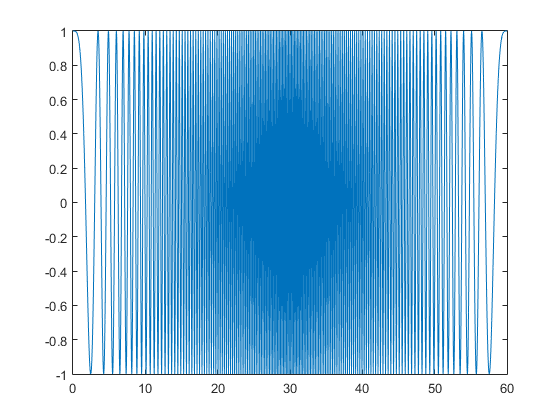
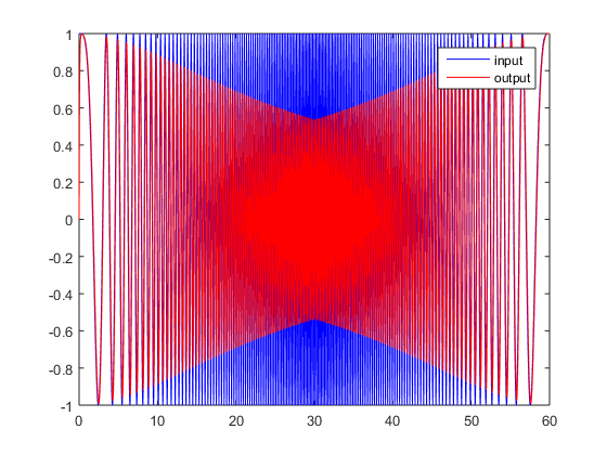
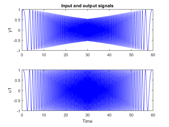
We run the script and yield a chirp signal shown in Figure 4a. Next, we set up the sampling time of the simulation to 1/10,000 of a second for the input block and the scope in Figure 2. We also save the simulation data from the scope as ScopeData in MATLAB workspace. These settings are shown in Figure 3. Then, we run the simulation and generate the output signal in Figure 4b.
3. System Identification
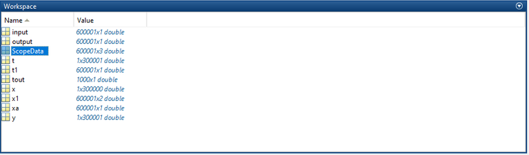
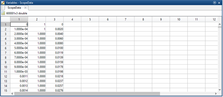
From the simulation, we acquire and save simulation data in MATLAB workspace as ScopeData. The file contains the time, input and output values from the simulation. Figure 5 shows ScopeData in MATLAB workspace and the data in ScopeData file.
From the ScopeData, we extract the input and output data from the array. We run the script:
input = ScopeData(:,2);
output = ScopeData(:,3);
to correctly assigned the input and output values to a specific variable. Next, we run
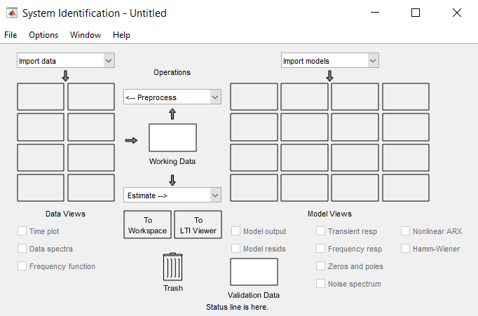
ident
in windows console to access the system identification tool in MATLAB. The system identification window is shown in Figure 6a.
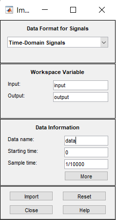
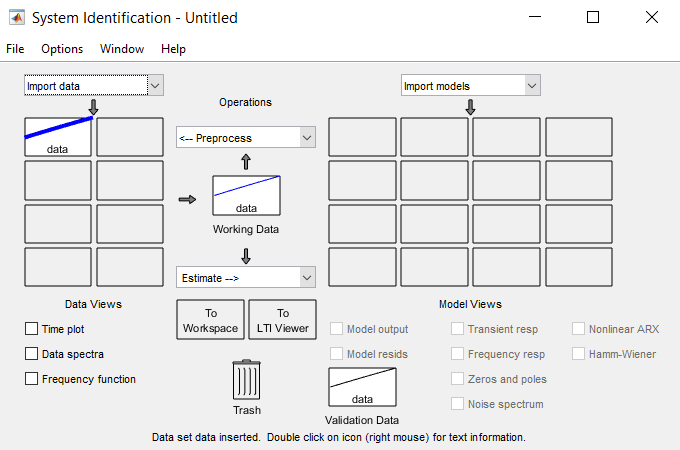
Next, we import the simulation data as data in the system identification windows. We also set the starting and sampling time to 0 and 1/10000 respectively, as shown in Figure 6b. To check the data, click the time plot and it displays Figure 7a.
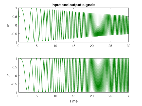
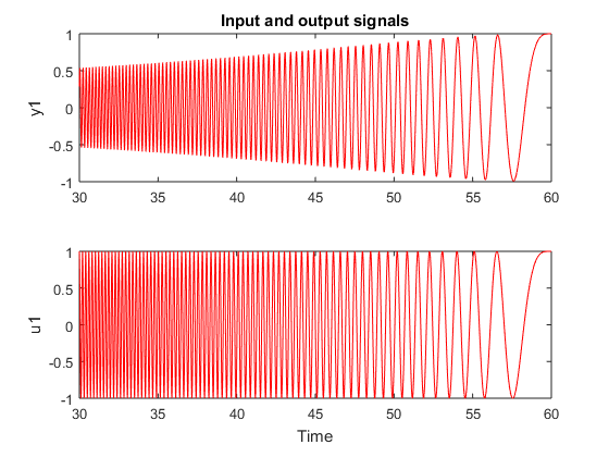
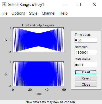
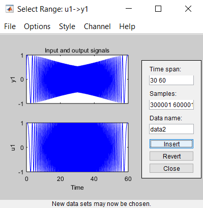
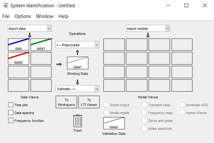
Then, we extract a working and validation data from data by setting up a different range for both data samples. We set the the time frame of the working data to 0 ≤ t ≤ 30 by accessing the drop down menu in preprocess and click on select range. We name the working data as data1. The setting for data1 is shown in Figure 8a. For the validation data, we set it to 30 ≤ t ≤ 60 and name it as data2. The setting for data1 and data2 is shown in Figure 8a and 8b respectively. After importing the data to system identification window, drag data1 to working data and data2 to validation data, as shown in Figure 8c. The time plot for data1 and data2 are shown in Figure 7b and 7c respectively.
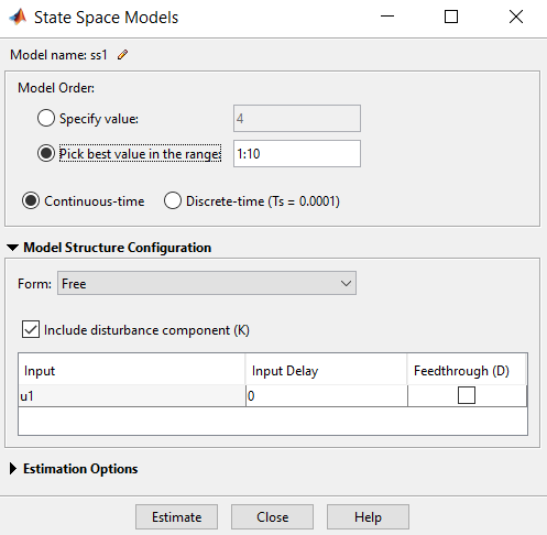
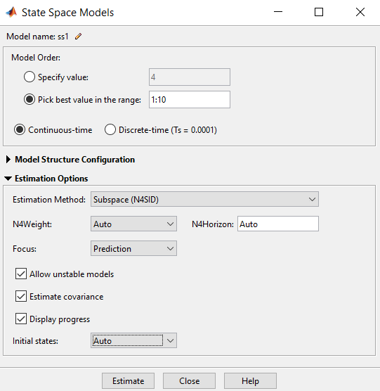
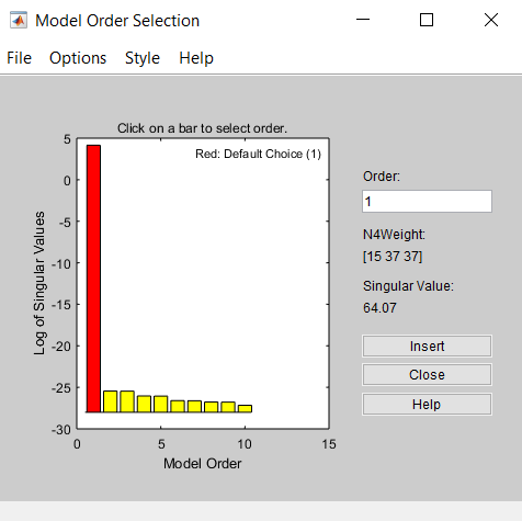
Lastly, we create the system model by clicking on the drop down menu in estimate and select state space model. In the state space model window as shown in Figure 9, set the model according to the settings in Figure 9 and click estimate. The system estimates the model order and rank based on its singular values, as shown in Figure 10. The system returns 10 model order for the simulation data. We choose the recommended model order and click insert to import the state space model into the system identification window.
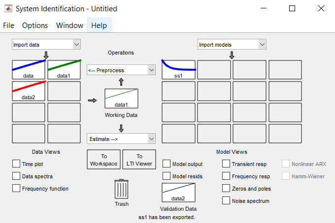
The state space model, ss1, is now in the system identification as shown in Figure 13. We check the model output, transient response, frequency response, and zeros and poles for the estimated state space model.
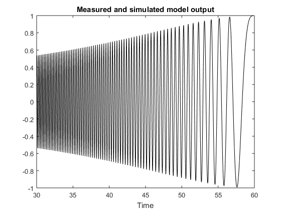
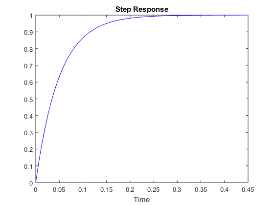
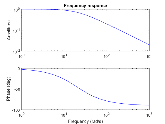
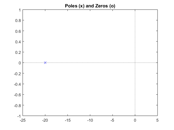
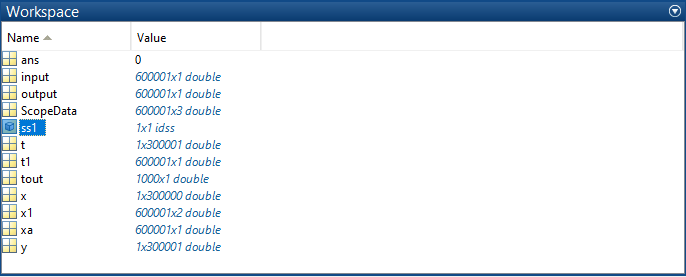
In Figure 12a, the state space model scores a 100% curve fitting between the measured and simulated model output. This suggest that the model correctly estimates the model from the simulation data. Other responses of the state space model are plotted in Figure 12. After checking the system output and responses, we imported the state space model to the MATLAB workspace by dragging it to workspace. Figure 13 shows ss1 is in MATLAB workspace.
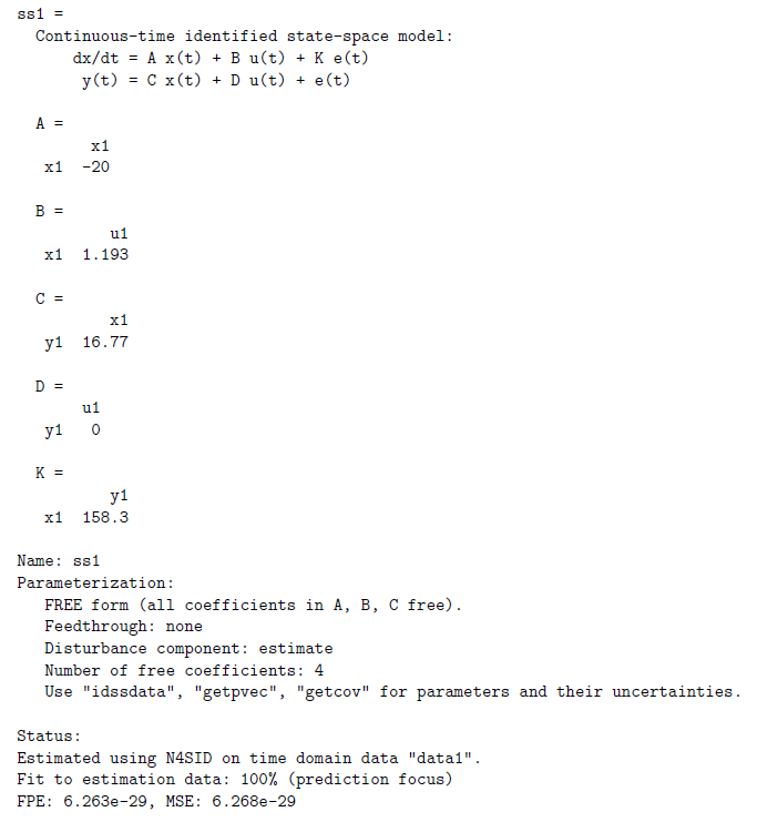
We run ss1 in windows console to generate the state space model of the system. The state model is
4. Validating the Transfer Function
In this section, we validate the transfer function in equation (1) to the transfer function generated by system identification using MATLAB and Simulink. We run
tf(ss1)
in windows console and get the transfer function from system identification as
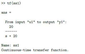
The transfer function from system identification is not in the same order as to the transfer function in equation (1) but numerically both transfer function yield to same response. Simplifying equation(1), we get
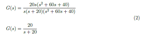
The first order model of the transfer function in equation (2) is equal to the transfer function from system identification. Thus, we validate that derived transfer function was correct.
5. Conclusion
In this paper, we are able to validate the transfer function in equation (1) and perform system identification using MATLAB and Simulink. We observed that system identification models system accurately from a set of input and output signal. In this paper, system identification methodology was able to derived the transfer function of the system from the simulation data in Simulink. It is a powerful tool in solving for the system models of systems without known characteristics and internal parameters. Also, it has a high accuracy in generating the estimated models.
6. References
[1] Norman S. Nise. Control Systems Engineering (7th. ed.). 2015. John Wiley & Sons, Inc., USA.
[3] Bishop, Robert H., and Richard C. Dorf. "Modern control systems." (2017).
[5] Ljung, Lennart. (2011). System Identification Toolbox for use with MATLAB. 21.
(Note: All images in the text is created by the author (@juecoree) except those with separate citation.)
If your interested in the modelling of the system transfer function in the text, read the previous post on:
1. State Space Model and System Transfer Functions
Posted with STEMGeeks
Posted with STEMGeeks
Thanks for your contribution to the STEMsocial community. Feel free to join us on discord to get to know the rest of us!
Please consider supporting our funding proposal, approving our witness (@stem.witness) or delegating to the @stemsocial account (for some ROI).
Please consider using the STEMsocial app app and including @stemsocial as a beneficiary to get a stronger support.