1. Introduction
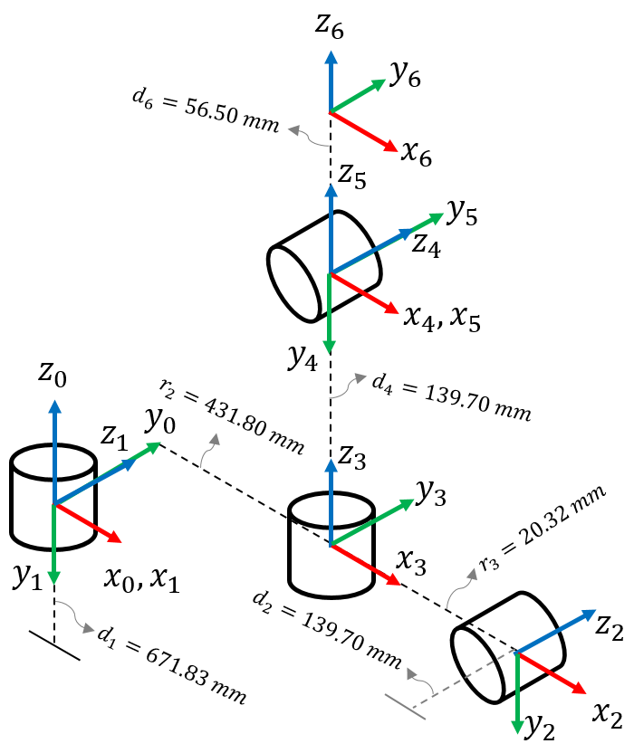
| Frame | θ | α | r | d |
|---|---|---|---|---|
| 1 | θ 1 | -90o | 0 | 671.83 mm |
| 2 | θ 2 | 0o | 431.80 mm | 139.70 mm |
| 3 | θ 3 | 90o | -20.32 mm | 0 |
| 4 | θ 4 | -90o | 0 | 431.80 mm |
| 5 | θ 5 | 90o | 0 | 0 |
| 6 | θ 6 | 0o | 0 | 56.50 mm |
In this paper, we derived the inverse kinematic of a PUMA 560 robot manipulator by decoupling method. We initially solve the joint angles from frame 0 to frame 3 and apply forward kinematics to build the homogeneous transformation matrix T03. This is discussed in section 2. For the joint angles in frame 4 to frame 5, we derive the equation defining the transformation matrix T36 and peg the resulting values from the dot product between the inverse of T03 and the transformation matrix T06 of the end-effector.
Furthermore, the inverse kinematic equation in section 2 is implemented in MATLAB. We evaluate solution of the inverse kinematic for PUMA 560 robot manipulator by comparing the result of fPUMA and iPUMA functions. The joint angles from the iPUMA function must be close to initiallize angle or to the end-effector in the fPUMA function.
2. Methods
2.1 Modelling of the Inverse Kinematics Equations
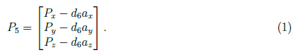
In inverse kinematic problem, we find a solution θ given a set of position and orientation of the end-effector. For PUMA 560 robot manipulator, we are given the DH model T06 which contains the orientation (rotation matrix) and the position (displacement matrix) of the end-effector. The angles at each joint is determined by decoupling the PUMA 560 robot manipulator. We initial solve the position (P5x, P5y, P5z) of the frame 5 and used these coordinate values to determine the angles (θ1, θ2, θ3) at the first three joint.
We start by determining the position of the frame 5 as shown in Figure 1. That is
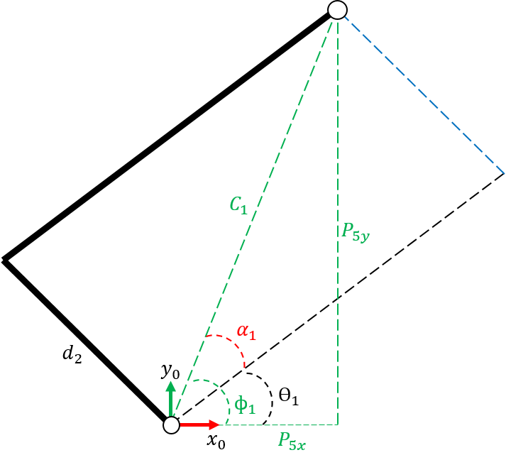
Next, we solve the angles at the first three joints by viewing PUMA 560 robot manipulator movement across x0 − y0 and x0 − z0 planes. In Figure 2, the joint angle θ1 is defined by the difference between angles φ1 and α1. The angle α1 is defined as
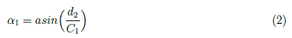
where
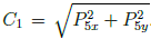
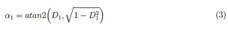
Equation (2) can be expressed in terms of atan2 function. We define
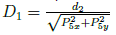
and yield
The angle φ1 is defined as

The joint angle θ1 is derived as

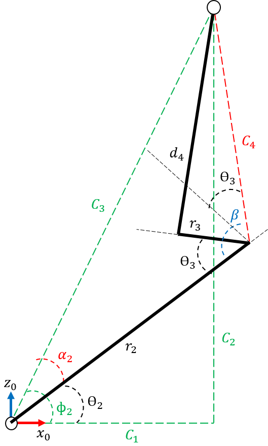
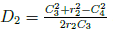
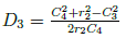
In Figure 3, we derived the equations to solve for the joint angles θ1 and θ2. We define the distances
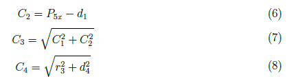
and apply cosine law to determine angles, α2 and β. We get the equations
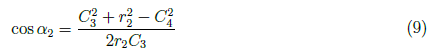
and
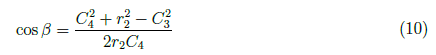
that gives the cosine value of α and β. We set
and
to define
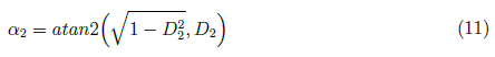
and
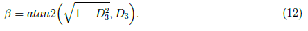
The angle φ2 is determined by

The joint angle θ2 is the difference between angles φ2 and α2 as shown in Figure 3. That is

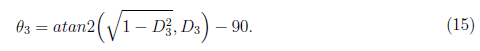
For the joint angle θ3, we have
After we obtain the angles at the first three joints, we used the angles to solve for the forward kinematics for frame 0 to frame 3. We solve the homogeneous transformation matrix T36 for frame 3 to frame 6 by taking the dot product between T06 and the inverse of T03. In general, DH model for 6 degrees of freedom manipulator is defined as

We can simplify the model to T06 = T03T36 and define

The angles at joint 4 to 6 is determine by deriving a set of equations from the homogeneous transformation matrix T36. The rotation matrix R36 holds the orientation of the end-effector in reference to frame 3. That is
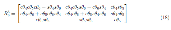
where the notation, sθ = sin θ and cθ = cos θ, is adapted. The R36 is a component in the homogeneous transformation matrix T36. We derived the joint angles θ4, θ5 and θ6 by equating the numerical values of T36 in equation (26).
We obtain the joint angle θ4 by
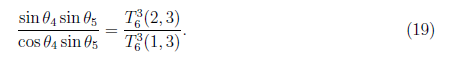
The joint angle θ4 is defined as

For joint angle θ5, we have cos θ5 = T36(3, 3) and used this equation to find θ5 in term of atan2 function. The joint θ5 is defined as

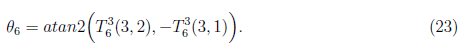
Lastly, the joint angle θ6 is derived by
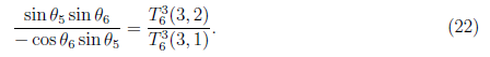
We have the joint angle θ6 as
2.2 MATLAB Implementation
In this section, we implement the derived inverse kinematic equations for PUMA 560 robot manipulator. We start by initializing the homogeneous transformation matrix T06 and the position of frame 5.
%DH parameter
A =  [-90 0 90 -90 90 0] ; %twist angle
r = [0 431.80 -20.32 0 0 0]; %offset as to xn
d = [671.83 139.70 0 431.80 0 56.50]; %offset as to z(n-1)
%DH model
T0_6 = [nx ox ax Px; ny oy ay Py; nz oz az Pz; 0 0 0 1];
% Joint 5 position
P = [Px-56.50*ax; Py-56.50*ay; Pz-56.50*az];
Next, we implement the equations to solve the joint angles θ1, θ2 and θ3 from the previous section. The MATLAB script is shown in listing 2.
%Determining Joint angles for frames 1,2,and 3
C1 = sqrt(P(1)^2+P(2)^2);
C2 = P(3)-d(1);
C3 = sqrt(C1^2+C2^2);
C4 = sqrt(r(3)^2+d(4)^2);
D1 = d(2)/C1;
D2 = (C3^2+r(2)^2-C4^2)/(2*r(2)*C3);
D3 = (r(2)^2+C4^2-C3^2)/(2*r(2)*C4);

a1 = atan2d(D1,sqrt(abs(1-D1^2)));
a2 = atan2d(sqrt(abs(1-D2^2)),D2);
b = atan2d(sqrt(abs(1-D3^2)),D3);
p1 = atan2d(P(2),P(1));
p2 = atan2d(C2,C1);
%Joint angles: theta_1, theta_2, and theta_3
J = [p1-a1 round(a2-p2) round(b-90)];
Then, we write a script to solve the forward kinematics for frame 0 to frame 6 and the homogeneous transformation matrix T36. The script is in listing 3.
%Apply forward kinematics at first three joints
T = [];
for n = 1:3
    matT = [cosd(J(n)) -sind(J(n))*cosd(A(n)) ...
            sind(J(n))*sind(A(n)) r(n)*cosd(J(n));
            sind(J(n)) cosd(J(n))*cosd(A(n)) ...
            -cosd(J(n))*sind(A(n)) r(n)*sind(J(n));
            0 sind(A(n)) cosd(A(n)) d(n);
            0 0 0 1];
        T = [T; {matT}];
end
T0_3 = T{1}*T{2}*T{3};
T3_6 = inv(T0_3)*T0_6;
Hence we already have the transformation matrix T36, we implement the equations to solve for the joint angles θ4, θ5 and θ6, as shown in listing 4.
%Joint angle: theta_4, theta_5, and theta_6
J4 = round(atan2d(T3_6(2,3),T3_6(1,3)));
J5 = round(atan2d(sqrt(abs(1-T3_6(3,3)^2)),T3_6(3,3)));
J6 = atan2d(T3_6(3,2),-T3_6(3,1));
Lastly, we solve the forward kinematics given the generated angles in the previous step and display a three-dimensional plot of the robot links and rotation.
All script discussed earlier was compiled to iPUMA function. The function accounts all derived equations for the inverse kinematics of PUMA 560 robot manipulator. The orientation as to the x-axis, y-axis and z-axis, and position of the end-effector are the input of the iPUMA function. Afterwhich, we compare the resulting angles and plot to the forward kinematics of PUMA 560 robot manipulator. This is to check if the derived equation arrived to the same end-effector point as generated by the forward kinematic model. The
full MATLAB script is shown in listing 5.
function iPUMA(nx, ny, nz, ox, oy, oz, ax, ay, az, Px, Py, Pz)
%input: end-effector position
%ouput: joint angles at each frames

%initial condition: iPUMA(1,0,0,0,1,0,0,0,1,411.50,139.70,1160.10)
format compact
format short
%DH parameter
A =  [-90 0 90 -90 90 0] ; %twist angle
r = [0 431.80 -20.32 0 0 0]; %offset as to xn
d = [671.83 139.70 0 431.80 0 56.50]; %offset as to z(n-1)
%DH model
T0_6 = [nx ox ax Px; ny oy ay Py; nz oz az Pz; 0 0 0 1];
% Joint 5 position
P = [Px-56.50*ax; Py-56.50*ay; Pz-56.50*az];

%Determining Joint angles for frames 1,2,and 3
C1 = sqrt(P(1)^2+P(2)^2);
C2 = P(3)-d(1);
C3 = sqrt(C1^2+C2^2);
C4 = sqrt(r(3)^2+d(4)^2);
D1 = d(2)/C1;
D2 = (C3^2+r(2)^2-C4^2)/(2*r(2)*C3);
D3 = (r(2)^2+C4^2-C3^2)/(2*r(2)*C4);

a1 = atan2d(D1,sqrt(abs(1-D1^2)));
a2 = atan2d(sqrt(abs(1-D2^2)),D2);
b = atan2d(sqrt(abs(1-D3^2)),D3);
p1 = atan2d(P(2),P(1));
p2 = atan2d(C2,C1);
%Joint angles: theta_1, theta_2, and theta_3
J = [p1-a1 round(a2-p2) round(b-90)];

%Apply forward kinematics at first three joints
T = [];
for n = 1:3
    matT = [cosd(J(n)) -sind(J(n))*cosd(A(n)) ...
            sind(J(n))*sind(A(n)) r(n)*cosd(J(n));
            sind(J(n)) cosd(J(n))*cosd(A(n)) ...
            -cosd(J(n))*sind(A(n)) r(n)*sind(J(n));
            0 sind(A(n)) cosd(A(n)) d(n);
            0 0 0 1];
        T = [T; {matT}];
end
T0_3 = T{1}*T{2}*T{3};
T3_6 = inv(T0_3)*T0_6;

%Joint angle: theta_4, theta_5, and theta_6
J4 = round(atan2d(T3_6(2,3),T3_6(1,3)));
J5 = round(atan2d(sqrt(abs(1-T3_6(3,3)^2)),T3_6(3,3)));
J6 = atan2d(T3_6(3,2),-T3_6(3,1));

J = [J J4 J5 J6];
%Plotting the result
if J(1,1) >= -160 && J(1,1) <= 160 && J(1,2)>= -225 ...
        && J(1,2) <= 45 && J(1,3) >= -45 && J(1,3) <= 225 ...
        && J(1,4) >= -110 && J(1,4) <= 170 && J(1,5) >= -100 ...
        && J(1,5) <= 100 && J(1,6) >= -266 && J(1,6) <= 266
    T = [];
    for n = 1:6
        matT = [cosd(J(n)) -sind(J(n))*cosd(A(n)) ...
            sind(J(n))*sind(A(n)) r(n)*cosd(J(n));
            sind(J(n)) cosd(J(n))*cosd(A(n)) ...
            -cosd(J(n))*sind(A(n)) r(n)*sind(J(n));
            0 sind(A(n)) cosd(A(n)) d(n);
            0 0 0 1];
        T = [T; {matT}];
    end
    P = [];
    for i = 1:6
        if i == 1
            P = [P,{T{i}}];
        else
            matP = P{i-1}*T{i};
            P = [P, {matP}];
        end
    end
    x = [0 P{1}(1,4) P{1}(1,4) P{2}(1,4) ...
        P{3}(1,4) P{4}(1,4) P{5}(1,4) P{6}(1,4)];
    y = [0 P{1}(2,4) P{2}(2,4) P{2}(2,4) ...
        P{3}(2,4) P{4}(2,4) P{5}(2,4) P{6}(2,4)];
    z = [0 P{1}(3,4) P{1}(3,4) P{2}(3,4) ...
        P{3}(3,4) P{4}(3,4) P{5}(3,4) P{6}(3,4)];
    hold on
    grid on
    rotate3d on
    plot3([x(1) x(2)],[y(1) y(2)],[z(1) z(2)]...
        ,'Color','b','LineWidth',5)
    plot3([x(2) x(3)],[y(2) y(3)],[z(2) z(3)]...
        ,'Color','r','LineWidth',5)
    plot3([x(3) x(4)],[y(3) y(4)],[z(3) z(4)]...
        ,'Color','g','LineWidth',5)
    plot3([x(4) x(5)],[y(4) y(5)],[z(4) z(5)]...
        ,'Color','c','LineWidth',5)
    plot3([x(5) x(6)],[y(5) y(6)],[z(5) z(6)]...
        ,'Color','m','LineWidth',5)
    plot3([x(6) x(7)],[y(6) y(7)],[z(6) z(7)]...
        ,'Color','y','LineWidth',5)
    plot3([x(7) x(8)],[y(7) y(8)],[z(7) z(8)]...
        ,'Color','k','LineWidth',5)
    plot3(x,y,z,'o','Color','k')
    xlabel('x-axis')
    ylabel('y-axis')
    zlabel('z-axis');
    title('Inverse Kinematics of PUMA 560 Manipulator (6DoF)')
    view(0,0)
    disp('The joint angles  are:   ');
    fprintf('theta1 = %f, theta2 = %f, theta3 = %f '...
        ,J(1),J(2),J(3));
    fprintf('theta4 = %f, theta5 = %f, and theta6 = %f  '...
        ,J(4),J(5),J(6));
else
    disp('Resulting joint angles is out of range');
end
3. Result
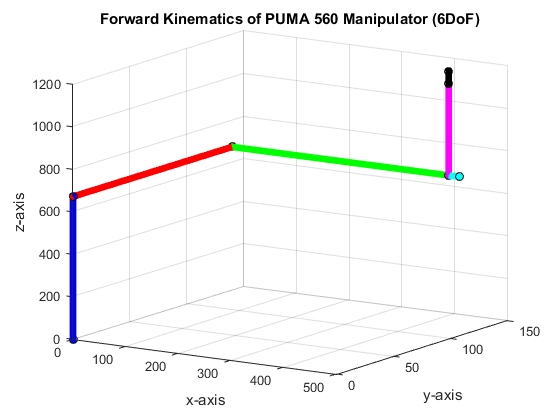
In this section, we present the result of the MATLAB implementation and validate it by comparing the it to the forward kinematic model. Initially, we set the input as
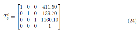
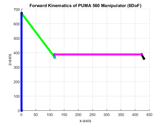
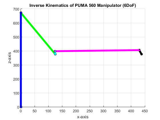
at initial condition where all joint angles are zero. The iPUMA function result to a joint angles: θ1 = 0, θ2= 0, θ3= 0, θ4 = 0, θ5 = 0, and θ6 = 0. Figure 4 shows the plot indicating the orientation and position of each frames of the robot manipulator. At initial condition, we observed that both the forward and inverse kinematics solution yield same values of joint angles, and orientation and position of end-effector.
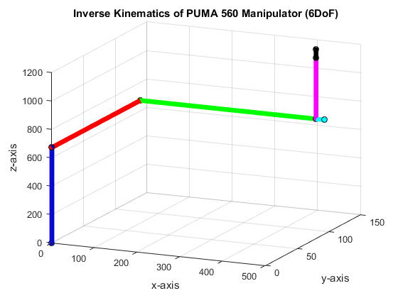
Next, we set the
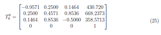
and have the joint angles as θ1 = 44.999712, θ2 = 43.000000, θ3 = 46.000000, θ4 = 44.000000, θ5 = 46.000000 and θ6 = 45.987531. We note that the input matrix is yield from all joint angles set to 45o. The resulting angles are close to 45o except for 1o to 2ooffset in joint angles. This is due to truncation and rounding off error in the inverse trigonometric functions in the code. Figure 5 shows the resulting plot.
Furthermore, we set are transformation matrix as
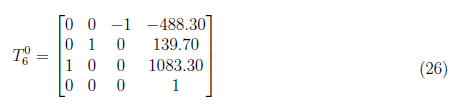
for all joint angles set to zero except θ2, = −90o.
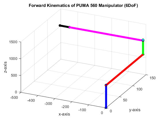
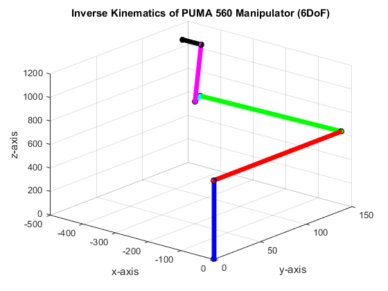
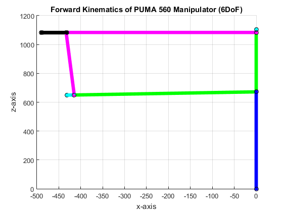
Figure 6: Results at zero except θ2, = −90o
The iPUMA function result to θ1 = 144.144160, θ2 = 3.000000, θ3 = 0.000000, θ4 = 36.000000, θ5 = 88.000000, and θ6 = 178.241701. For this simulation, it is evident that the angles are have large offset as to the actual angles for the given end-effector however the set of joint angles still reaches the same end-effector point as shown in Figure 6. This is unique to the solution of inverse kinematics. It generate multiple combination of angles that adhere to the given orientation and position of an end-effector.
4. Conclusion
In this paper, we modelled the inverse kinematics of PUMA 560 robot manipulator. We derived the equations of the joint angles by decoupling the PUMA 560 frames. We initial solve for frame 0 to frame 3 and then the last remaining frames. A detailed derivation of equations for the joint angles are in section 2. The inverse kinematic equations was implemented in MATLAB and verify the result by comparing it with the forward kinematics. In section 3, the iPUMA function generates the joint angle with minimal error. We also observed that in some cases, the angles generated are not the same with the basis but still reaches the same end-effector. Thus, inverse kinematic of a 6 degrees of freedom robot manipulator has multiple possible solution for a given orientation and position of the end-effector.
5. References
[1] Lynch, K. and F. Park. “Modern Robotics: Mechanics, Planning, and Control.” (2017).
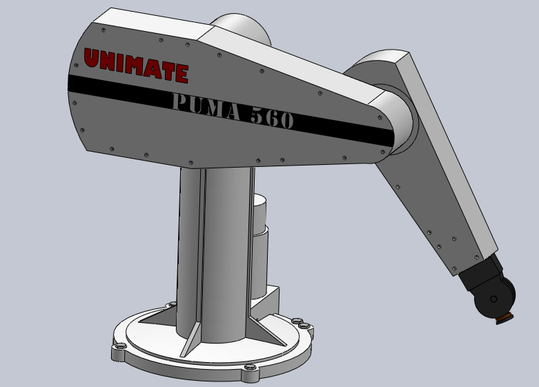
(Note: All images in the text are drawn by the author except those with attached citations. The cover 3D model of PUMA 560 is created by Gonzalo Loredo Neri and is free to download at grabcad.com))
If your interested with the forward and inverse kinematics of robots, check these post:
1. Forward Kinematics of PUMA 560 Robot using DH Method
2. Forward and inverse kinematics of 3R Planar Manipulator
Posted with STEMGeeks
Thanks for amazing post
Your welcome!