1. Introduction

In the succeeding sections, the modelling of these equations is discussed in detail. Aside from the equations, we implement a MATLAB code to generate response curves for for the state variables and output for zero input, zero state and the complete system response.
2. Time Domain Response
In this section, we solve for the time domain response of the system in Figure 1. The system has a state space model defined as
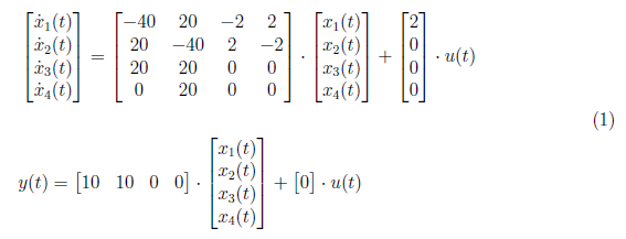
From the state space model, we defined state space equations in phase domain as
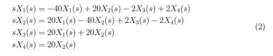
By equating the state space equations, we derived X1(s), X2(s), X3(s) and X4(s) as
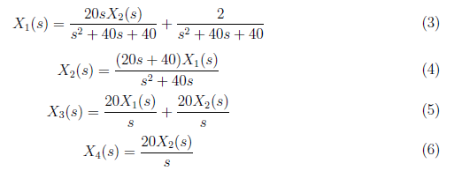
Substitute X2(s) to equation (3), and yield
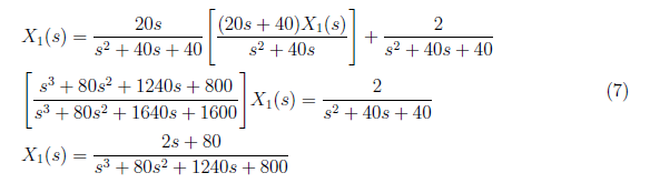
We solve the equivalent partial fraction for equation(7) which is defined as
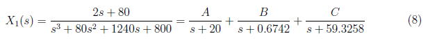
and by equating the coefficient, we derived these equations:
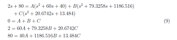
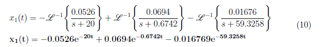
From the equation (9), we have A = −0.0526, B = 0.0694 and C = −0.01676. We substitute the values of A, B, C and D to equation (8) and apply inverse Laplace transform to get x1(t) as
For x2(t), we begin by substituting equation (3) to (4) and obtain
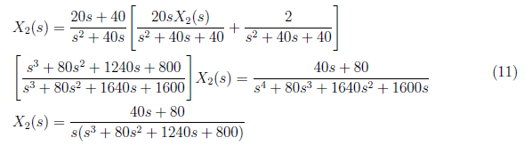
From equation (11), we set the partial fraction as

and by equating coefficients, we have these equations:
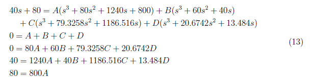
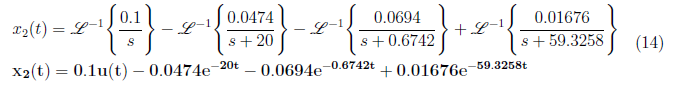
We get A = 0.1, B = −0.0474, C = −0.0694 and D = 0.01676 from the equation (13), . We substitute the values of A, B, C and D to equation (12) and apply inverse Laplace transform to get x2(t) as
For x3(t) and x4(t), substitute x1(t) and x2(t) to equations (5) and (6) and obtain

and

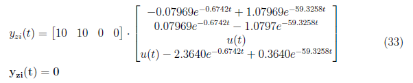
We defined zero input response for y(t) as

3. Zero input and Zero State Response
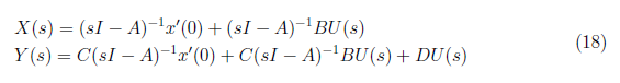
In this section, we derived the zero input and zero state response of the system. The zero input response is the system response to the initial condition when input is set to zero. The zero state response is the system response to the input when input is set to zero. The total system response is the sum of the zero input and zero state response and defined as
3.1 Zero Input
We derive the equation for zero input response from the state space equation in phase domain and set x'(0) = 1 for all state variables to have a non-zero response. The zero input response is defined as

We derived (sI − A)−1 in the previous paper. That is
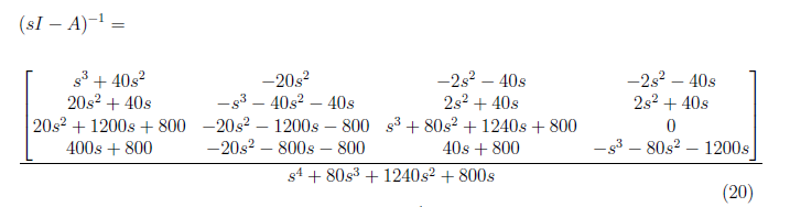
We substitute the initial condition and (sI − A)−1 to equation (19). We obtain
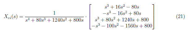
We apply inverse Laplace transform to Xzi to yield the zero input response. We initially simply the equation using partial fraction. This eases the complexity when we preform inverse Laplace transformation. We express X1(zi) in partial fraction as
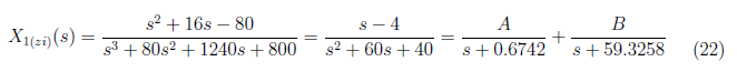
By equating coefficient, we determine these equations:
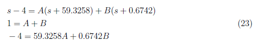
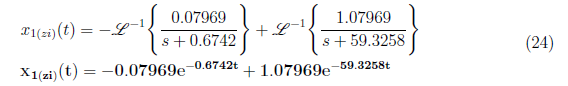
Substitute A = −0.07969 and B = 1.0797 to equation (22) and apply inverse Laplace to get x1(zi)(t) as
For x2(zi)(t), we solve for the partial fraction by

and by equating coefficient, we define these equations
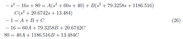
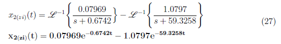
We get A = 0, B = 0.07969 and C = −1.0797 and substitute to equation (25). We have x2(zi) as
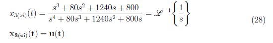
We simplify X3(zi)(s) and apply inverse Laplace transformation to yield
For x4(zi)(t), we initially determine the equivalent partial fraction which is defined by
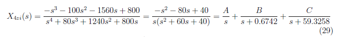
and by equating coefficient, we solve A, B and C from these equations
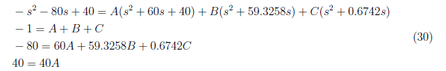
We substitute A = 1, B = −2.3640 and C = 0.3640 to equation (29) and apply inverse Laplace transform to get
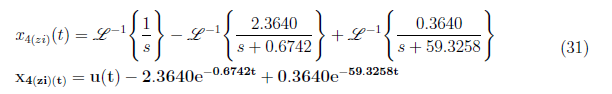
Thus, we have the zero input response model as
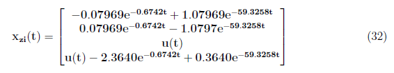
and
3.2 Zero State
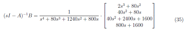
In this section, we derive the equation for zero state response from the state space equation in phase domain and assume unit step input, U(s) = 1/s. The zero state response is defined as

We take the dot product between (sI − A)−1 and B to yield
We derived Xzi(s) as
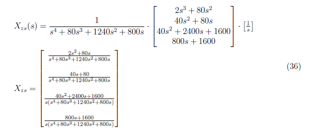
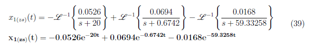
To determine the zero state response, we apply inverse Laplace transformation to the equation in each element in the Xzs(s) matrix. We express X1(zs)(s) in partial fraction as
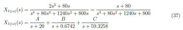
and by equating coefficient, we find A, B and S using these equations:
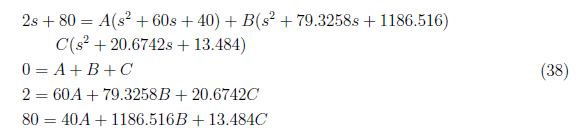
We have A = −0.0526, B = 0.0694 and C = −0.0168 and substitute it to equation (37). Afterwards, apply inverse Laplace transform and yield x1(zs)(t) as
For x2(zs)(t), we have partial fraction representation of X2(zs)(s) as
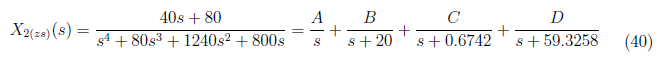
and we equate coefficient to form these equations
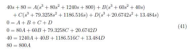
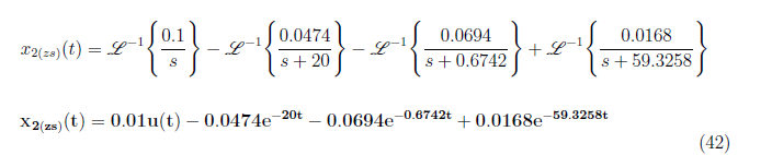
We have A = 0.1, B = −0.0474, C = −0.0694 and D = 0.0168 and substitute it to equation (40). We perform inverse Laplace transformation to X2zi(s) and get
For x3(zs)(t), we have partial fraction representation of X3(zs)(s) as
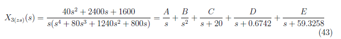
and by equating coefficcient, we get these equations:
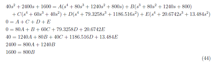
With A = −0.1 and B = 2, we can simplify the set of equations to
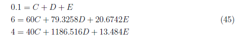
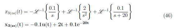
We obtain C = 0.1, D = 0 and E = 0 and substitute these values of to equation (43). Apply inverse Laplace transformation to the resulting equation and define x3(zs)(t) as
For x4(zs)(t), we have partial fraction representation of X4(zs)(s) as
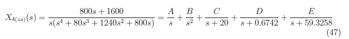
and by equating coefficient, we have these equations:
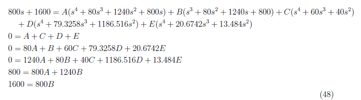
Simplifying the earlier equation by substituting A = −2.10 and B = 2 and we get
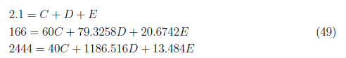
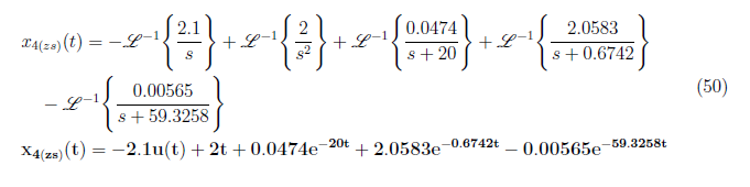
We have C = 0.0474, D = 2.0583 and E = −0.00565. We take thee inverse Laplace of X4(zs)(s) and derived x4(zs) (t)as
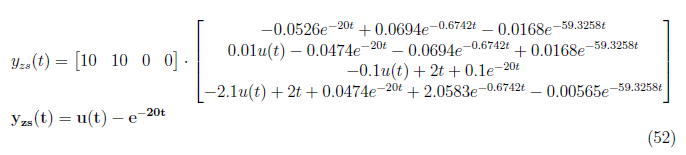
Thus, we have the zero state response model as
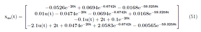
and
3.3 Complete System Response
The complete system response for a system is given by the summation of zero input and zero responses of the system. That is
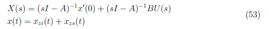
and
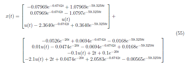
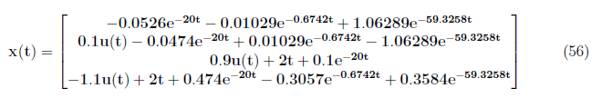
Substituting the values xzi(t) and xzs(t) to the complete system response equation, we obtain the complete state response x(t) as
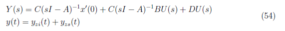
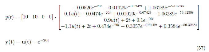
The complete output response y(t) is defined as
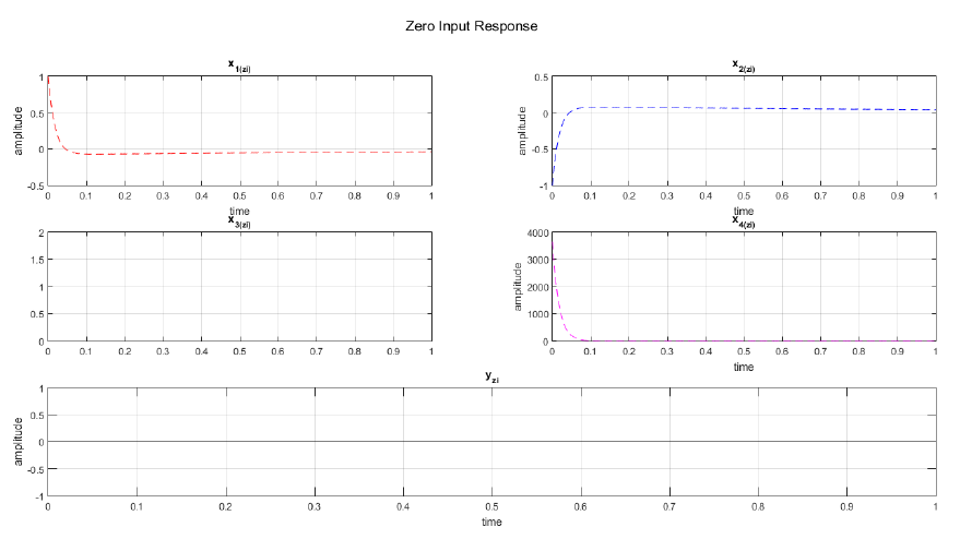
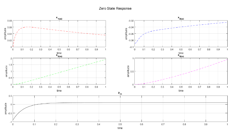
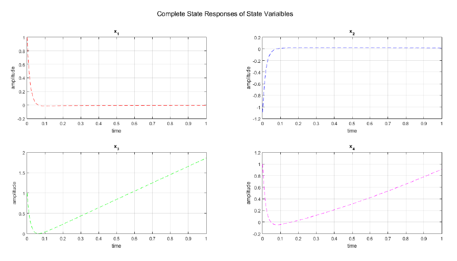
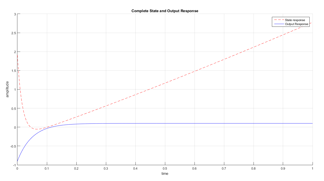
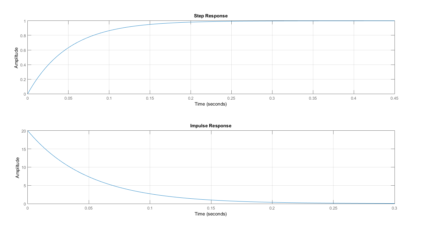
We implement the derived equations for zero input, zero state, complete state and output responses in MATLAB. As a result, we are able to plot and observed the responses of each variables. Figure 2 displays the zero input response curve of the each state variables and the output. As observed, no plot is showed in x2(zi) hence it is time invariant. The output yzi at zero input condition yields to zero amplitude response and time invariant. In Figure 3, the zero state response of each variables are shown while Figure 4 displays the complete state responses of each state variables. We plot the complete state and output responses as shown in Figure 5. We also display the step and impulse response of the system as shown in Figure 6.
The step response curve in Figure 6 is generated from the transfer function of the system. In section 2, we assumed a unit step input U(s) to derived the equations for time domain, zero-input and zero state response of the system. We verifies the output response by comparing it to the step response. As observed, the output y(t) has similar trend as to the step response. This validated that the equations are correctly modelled.
3.4 MATLAB Code
In this section, all the script needed to get the output and plot are listed. First, we define the state space model for the given system as shown in the code in Listing 1.
%state space model
A = [-40 20 -2 2;20 -40 2 -2; 20 20 0 0; 0 20  0 0];
B = [2; 0; 0; 0];
C = [10 10 0 0];
D = [0];
sys = ss(A,B,C,D);
[Num, Den] = ss2tf(A,B,C,D);
Gs = tf(Num,Den);
After, we implement the time-domain equations for each state variables. Also, we write a code to plot the responses at each variables. The code is presented in listing 2.
%input and time frame
u = 1;
t = 0:0.0001:1;

%zero input response
x1_zi = -0.07969*exp(-0.6742*t)+ 1.07969*exp(-59.3258*t);
x2_zi = 0.07969*exp(-0.6742*t)- 1.07969*exp(-59.3258*t);
x3_zi = u;
x4_zi = u-2.364*exp(-0.6742*t)+03640*exp(-59.3258*t);
y_zi = 10*x1_zi + 10*x2_zi;

%plotting zero input response
hold on
subplot(3,2,1)
plot(t, x1_zi, '--','Color', 'r', 'linewidth',);
xlabel('time')
ylabel('amplitude')
title('x_{1(zi)}')
grid on
subplot(3,2,2)
plot(t, x2_zi, '--','Color', 'b');
xlabel('time')
ylabel('amplitude')
title('x_{2(zi)}')
grid on
subplot(3,2,3)
plot(t, x3_zi, '--','Color', 'g');
title('x_{3(zi)}')
grid on
subplot(3,2,4)
plot(t, x4_zi, '--','Color', 'm');
xlabel('time')
ylabel('amplitude')
title('x_{4(zi)}')
grid on
subplot(3,2,[5,6])
plot(t, y_zi,'Color', 'k');
xlabel('time')
ylabel('amplitude')
title('y_{zi}')
grid on
suptitle('Zero Input Response')


%zero state response
x1_zs = -0.0526*exp(-20*t)+0.0694*exp(-0.6742*t)...
    -0.0168*exp(-59.3258*t);
x2_zs = 0.01*u-0.0474*exp(-20*t)-0.0694*exp(-0.6742*t)...
    +0.0168*exp(-59.3258*t);
x3_zs = -0.1*u+2*t+0.1*exp(-20*t);
x4_zs = -2.1*u+2*t+0.0474*exp(-20*t)+2.0583*exp(-0.6742*t)...
    -0.00565*exp(-59.3258*t);
y_zs = 10*x1_zs + 10*x2_zs;

%plotting zero state response
hold on
subplot(3,2,1)
plot(t, x1_zs, '--','Color', 'r');
xlabel('time')
ylabel('amplitude')
title('x_{1(zs)}')
grid on
subplot(3,2,2)
plot(t, x2_zs, '--','Color', 'b');
xlabel('time')
ylabel('amplitude')
title('x_{2(zs)}')
grid on
subplot(3,2,3)
plot(t, x3_zs, '--','Color', 'g');
xlabel('time')
ylabel('amplitude')
title('x_{3(zs)}')
grid on
subplot(3,2,4)
plot(t, x4_zs, '--','Color', 'm');
xlabel('time')
ylabel('amplitude')
title('x_{4(zs)}')
grid on
subplot(3,2,[5,6])
plot(t, y_zs,'Color', 'k');
xlabel('time')
ylabel('amplitude')
title('y_{zs}')
grid on
suptitle('Zero State Response')

%complete state and output response
x1 = x1_zi+x1_zs;
x2 = x2_zi+x2_zs;
x3 = x1_zi+x3_zs;
x4 = x1_zi+x4_zs;
x = x1+x2+x3+x4;
y = 10*x1+10*x2;

%plotting complete state response for each state variables
hold on
subplot(2,2,1)
plot(t, x1, '--','Color', 'r');
xlabel('time')
ylabel('amplitude')
title('x_{1}')
grid on
subplot(2,2,2)
plot(t, x2, '--','Color', 'b');
xlabel('time')
ylabel('amplitude')
title('x_{2}')
grid on
subplot(2,2,3)
plot(t, x3, '--','Color', 'g');
xlabel('time')
ylabel('amplitude')
title('x_{3}')
grid on
subplot(2,2,4)
plot(t, x4, '--','Color', 'm');
xlabel('time')
ylabel('amplitude')
title('x_{4}')
grid on
suptitle('Complete State Responses of State Varialbles')


%plotting complete state and output response
hold on
plot(t,x,'--','Color','r');
plot(t,y,'Color','b');
title('Complete State and Output Response');
xlabel('time')
ylabel('amplitude')
legend('State response', 'Output Response');
grid on
Then, we plot the step and impulse response of the system as shown in Listing 3.
%plotting step and impulse response
hold on
subplot(2,1,1)
step(Gs);
title('Step Response')
grid on
subplot(2,1,2)
impulse(Gs);
title('Impulse Response')
grid on
4. Conclusion
In this paper, we modelled an equation for the time domain, zero input and zero state response of the system in Figure 1. Also, we evaluate the the derived solutions by plotting the response curve of each state variables and the output. In general, zero input and zero state response defines the total system response in time domain. The zero input response was initialized with x'(0) = 1 for all state variables to yield to a response value peg to the zero input.
On the other hand, the zero state solution yields to response values that is peg to the initial condition of the system. Furthermore, we note a similar equation in the output y(t) and zero state output response yzs(t). The complete response of the system is the sum of the zero input and zero state response of the system.
5. References
[1] Norman S. Nise. Control Systems Engineering (7th. ed.). 2015. John Wiley & Sons, Inc., USA.
[3] Bishop, Robert H., and Richard C. Dorf. "Modern control systems." (2017).
(Note: All images in the text is created by the author (@juecoree) except those with separate citation.)
Interested in my previous articles, here is a list:
Control System:
1. State Space Model and System Transfer Functions
2. System Identification using MATLAB and Simulink
Robotics:
1. Forward and Reverse Kinematics for 3R Planar Manipulator
2. Forward Kinematics of PUMA 560 Robot using DH Method
3. Inverse Kinematics of PUMA 560 robot
!discovery 45
This post was shared and voted inside the discord by the curators team of discovery-it
Join our community! hive-193212
Discovery-it is also a Witness, vote for us here
Delegate to us for passive income. Check our 80% fee-back Program
Thanks for your contribution to the STEMsocial community. Feel free to join us on discord to get to know the rest of us!
Please consider supporting our funding proposal, approving our witness (@stem.witness) or delegating to the @stemsocial account (for some ROI).
Please consider using the STEMsocial app app and including @stemsocial as a beneficiary to get a stronger support.