1. Introduction
The system can be represented with different state variables even though the transfer function relating the output to the input remains the same. The various forms of the state space equations yield from the transfer function, drawing signal flow graphs, and deriving equations from signal flow graphs. These systems are called similar system.

In this paper, we explored and derived the equations for the decoupled representation of the system using similarity transformation. Similarity transformation projects a new system, input, output, and feedforward matrix of the system for a new basis vector. In this paper, we highlighted the derivation of the transformation matrix , P, and the decoupled system equations. Also, the signal flow graph for the decoupled system is presented.
The given system consist of a voltage input, u(t), resistors, R1, R2 and R3, inductors, L1 and L2, and capacitors, C1 and C2. The output y(t) is equal to the voltage across the resistor, R2. The values of each elements are R1, R2, R3 = 10 Ω, L1, L2 = 0.5 H and C1, C2 = 50 mF. The state space model of the system in Figure 1 is given by
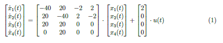
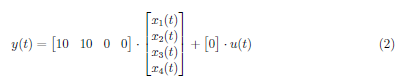
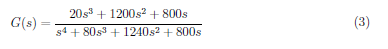
and a transfer function defined as
In the succeeding sections, the process of decoupling a system in state space is discussed in details. The paper implement some analytical solution in MATLAB for ease of computation and derivation of numerical values in the discussion.
2. Decoupling a System in State Space
Diagonal system matrix define the state space equation as a function of one state variable. This allow easier analysis hence each differential equation is solved independently of the other equations. The equations are said to be decoupled. There are two ways to decoupled a system in state space. We used partial fraction and signal flow graphs from the transfer function or by similarity transformation of the state space model. In this paper, the latter is adapted.
2.1 Finding the Transformation Matrix, P
In this section, we formed the transformation matrix, P, from the vector quantities expressed in the system matrix. Initially, we calculate the eigenvalues and eigenvectors of the system matrix. We solve the eigenvalues using det (λI − A) = 0 as derived from Ax = λx. The eigenvector is denoted as x. The eigenvalues are defined as
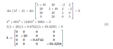
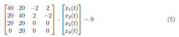
For each of the eigenvalues, plug back in to the (λI − A) and solve the associated system of equation to determine the eigenvectors. We have four set of homogeneous system of equations for each eigenvalues and using Gaussian elimination, we solve for the eigenvector. For λ1 = 0, solve:
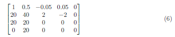
We start with dividing the first row A1 by the A
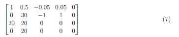
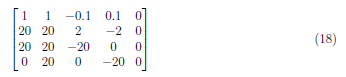
To zero the A2,1, we perform (A2 − 20) · A1 → A2, producing the following matrix:
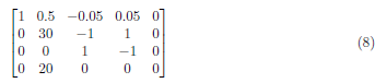
Apply (A3 − 20) · A1 → A3 and get
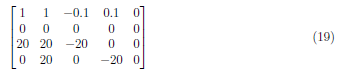
At A2 divide each element by 30, and have the matrix:
Perform (A4 − 20) · A1 → A4 and form the matrix:
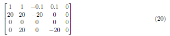
To zero A4, we subtracting A3 to A4 and get the matrix:
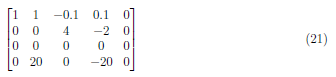
To zero the A2,3, we apply (A3 − (−0.3333)A2) → A2 and obtain
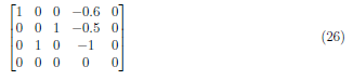
Next, we perform (A1 − (−0.5)A3) → A1 and have the matrix:
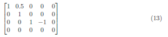
Then, apply (A1 − 0.5A2) → A1, and the equivalent homogeneous system of equations is
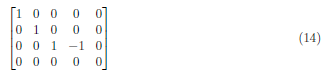
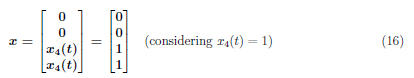
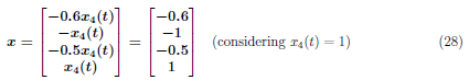
This has a general solution

Eigenvectors associated with the eigenvalue (λ1 = 0) are
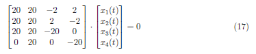
For λ2 = −20, solve:
We divide A1 by 20 and get
To zero the value at A2,1, we apply (A2 − 20A1) → A2 and form the matrix:
Interchange A2 and A3(A3↔A2) to obtain the matrix:
Apply (A2− 20)·A1→A2 and get
Divide A2 by 4 and have the matrix:
Interchange A3 and A4(A4↔A3) to have
Divide A3 by 20 and form the matrix:
Subtract A3 to A2 to obtain
Apply (A1−(−0.1)·A2→A1 and get
This has a general solution

Eigenvectors associated with the eigenvalue (λ2 = −20) are
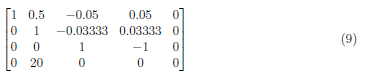
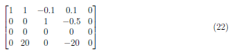
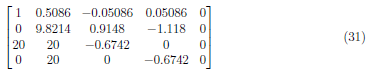
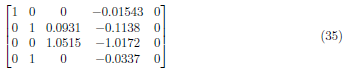
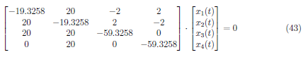
For λ3 = −0.6742, solve:
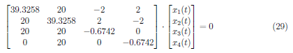
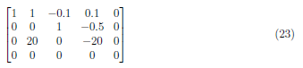
We start by dividing 39.3258 to A1 and obtain the matrix:
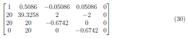
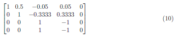
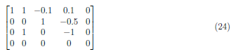
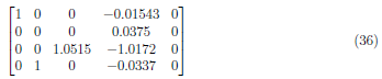
Perform (A2 − 20) · A1 → A2 and get
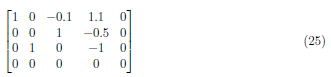
Divide A2 by 9.8214 and obtain
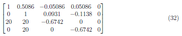
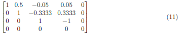
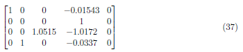
To zero A3,1, we apply (A3 − 20) · A1 → A3 and form the matrix:
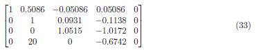
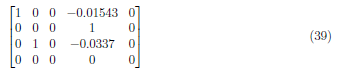
Divide A3 by 20 to form the matrix:
Apply (A1 − 0.5086) · A4 → A1 and obtain the matrix:
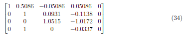
Apply (A2 − 1) · A4 → A2 and get
Divide A2 by 0.0375 to form the matrix:
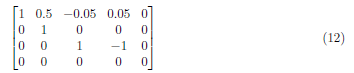
To zero A3,4, we apply (A3 − (−1.017)) · A2 → A3 to have the matrix as
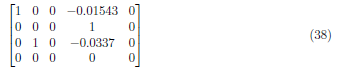
Interchange A3 and A4 and get
Interchange A3 and A2 and get
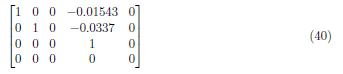
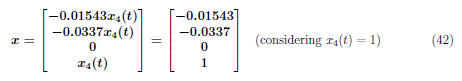
This has a general solution

Eigenvectors associated with the eigenvalue (λ3 = −0.6742) are
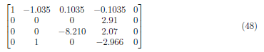
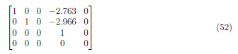
For λ4 = −59.3258, solve:
We divide A1 and A2 by -19.3258 to form the matrix:
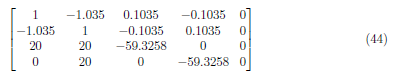
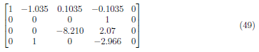
To make A2,1 = 0, we perform (A2 − (−1.035)) · A1 → A2 and obtain
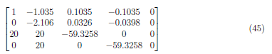
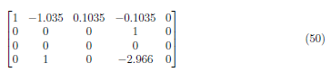
To make A3,1 = 0, we perform (A3 − (20)) · A1 → A3 and obtain
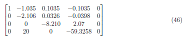
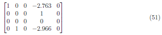
Divide A4 by 20 and A2 by -2.106 to form the matrix:
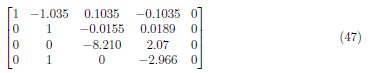
To make A2,2 = 0, perform (A2 − 1) · A4 → A2 and get
Divide A2 by 2.91 to have the matrix:
Apply (A3 − 2.07) · A2 → A3 to get the matrix:
Next, perform (A1 − (−1.035)) · A4 → A1 to obtain
We interchange the rows and form the matrix:
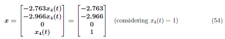
This has a general solution

Eigenvectors associated with the eigenvalue (λ4 = −59.3258) are
Hence there are multiple possible eigenvectors for the a given eigenvalues, we use MATLAB to find the best eigenvectors that described the system. We run listing 1 in MATLAB to generate the eigenvectors V and eigenvalues D.
%state space model of the system
 A = [=40 20 =2 2 ; 20 =40 2 =2 ; 20 20 0 0 ; 0 20 0 0 ] ;
B = [ 2 ; 0 ; 0 ; 0 ] ;
C = [ 1 0 10 0 0 ] ;
D = [ 0 ] ;

%solving the eigenvalues and eigenvectors
[V,D] = e i g (A) ;
The code generates the following eigenvector and eigenvalues:
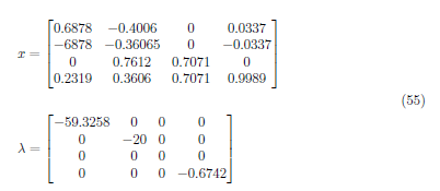
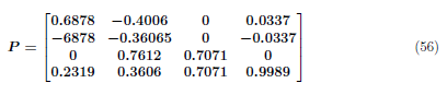
The transformation matrix, P, is the eigenvectors of the given system which is described in equation (55). We defined the transformation matrix, P, as
2.2 Diagonalizing a system in state space
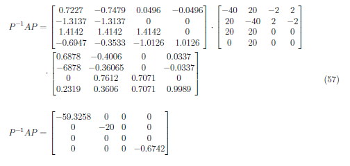
In this section, we used the transformation matrix to define the similar system’s system matrix, input matrix and output matrix. Using similarity transformation, we defined the new system matrix as
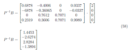
The input matrix is defined as
Then, the output matrix is defined as
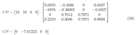
From the matrices earlier, we defined the transformed system as
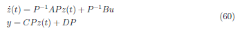
where Pz(t) = x(t) and z(t) is the transformed state variable. Plugging in the matrices, the transformed system is defined as
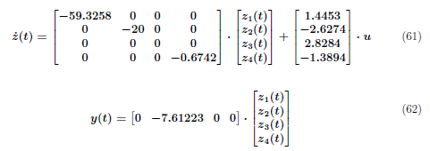
Thus, a diagonal system matrix in equation (61) and (62) denote that the system is decoupled.
2.3 Transfer Function
Decoupling a system in state space gives a different model of the system but have similar response by means of similarity transformation. In similarity transformation, we defined the similar system which is expressed in terms of a new basis vector. The transfer function of the given system never changes as to the system representation, whether state space, time domain or decoupled.
In this section, we derive the transfer function of the similar system and compare it with the previously derived transfer function. The new transfer function is generated by running the MATLAB code in listing 2.
%transformed system
2 nA = in v (V) *A*V;
3 nB = in v (V) *B;
4 nC = C*V;
5 nD = [ 0 ] ;
6
7 %transfer functio n
8 s y s = s s (nA, nB, nC, nD, 0 . 2 5 ) ;
9 [num, den ] = s s 2 t f (nA, nB, nC, nD) ;
The transfer function (decoupled) is defined as
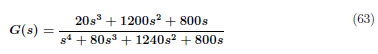
The transfer function in equation (63) is the same as to the transfer function from the state space model in equation (3). Thus, the decoupled system equations in equation (61) and (62) is correctly modelled and has similar response to the state space model (coupled) of the system in Figure 1.
2.4 Signal Flow Graph
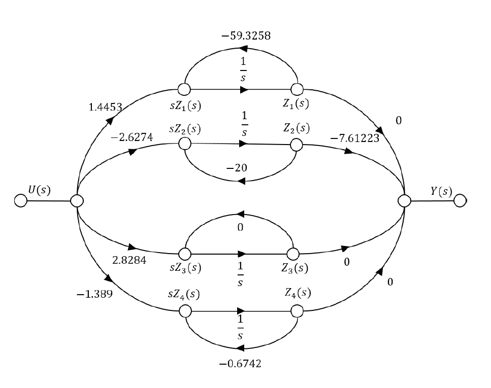
We apply Laplace transform to equation (61) and (62) and have the decoupled system equation in phase domain as
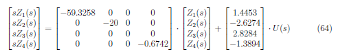
These equations yield to a signal flow graph in Figure 2.
3 Conclusion
In this paper, we explore and derived the decoupled system equation of the system using similarity transformation. In section 2, a step-by-step process was presented on how to decouple a system in state space. Decoupling a system in state space never changes the system response (transfer function) but only give a different model for the given system. The state space model of a system is said to have multiple representation. These system are similar system. The given system in Figure 1 has a decoupled system defined in equation (61) and (62). It is clearly implied in the paper that coupled and decoupled system have the same transfer function but differently portrayed in the equations.
4. References
[1] Norman S. Nise. Control Systems Engineering (7th. ed.). 2015. John Wiley & Sons, Inc., USA.
[3] Bishop, Robert H., and Richard C. Dorf. "Modern control systems." (2017).
(Note: All images in the text is created by the author (@juecoree) except those with separate citation.)
Interested in my previous articles, here is a list:
Control System:
1. State Space Model and System Transfer Functions
2. System Identification using MATLAB and Simulink
3. Time Domain, Zero Input and Zero State Response
Robotics:
1. Forward and Reverse Kinematics for 3R Planar Manipulator
2. Forward Kinematics of PUMA 560 Robot using DH Method
3. Inverse Kinematics of PUMA 560 robot
Wow!
Congratulations @juecoree! You received a personal badge!
Wait until the end of Power Up Day to find out the size of your Power-Bee.
May the Hive Power be with you!
You can view your badges on your board and compare yourself to others in the Ranking
Do not miss the last post from @hivebuzz:
Congratulations @juecoree! You received a personal badge!
Participate in the next Power Up Day and try to power-up more HIVE to get a bigger Power-Bee.
May the Hive Power be with you!
You can view your badges on your board and compare yourself to others in the Ranking
Do not miss the last post from @hivebuzz:
Thanks for your contribution to the STEMsocial community. Feel free to join us on discord to get to know the rest of us!
Please consider supporting our funding proposal, approving our witness (@stem.witness) or delegating to the @stemsocial account (for some ROI).
Please consider using the STEMsocial app app and including @stemsocial as a beneficiary to get a stronger support.